|
|
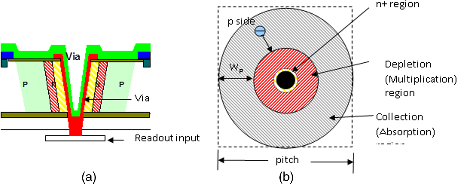
1.IntroductionA flash imaging lidar is a laser-based 3-D imaging system in which a large area is illuminated by each laser pulse and a focal plane array (FPA) is used to simultaneously detect light from thousands of adjacent directions. Mapping and 2-D/3-D imaging are examples of applications for such systems. To make these systems as robust as possible, and to reduce the amount of laser power required, receivers in flash lidar systems typically employ some form of gain. One approach is to provide gain in the incident optical signal (photon gain, one example being fiber amplifiers). Another approach, which is a major subject for this paper, is charge gain inside the detector after photon detection has occurred. Charge gain processes inside detectors exploit the ability to accelerate charged particles in an applied electric field to amplify the number of charge carriers through energetic collisions. One example is photoemissive detectors in which a primary electron generated by the incident absorbed photon is liberated from the detector photocathode, accelerated through an evacuated space by an applied electric field, and then impacted on a target material, generating additional secondary charge carriers from the primary carrier’s kinetic energy. A second type of detector charge gain process is impact ionization inside an avalanche photodiode (APD) in which the primary photoelectrons do not leave the detector material but undergo ionizing collisions within the semiconductor crystal in a high-electric field region of a reverse-biased diode junction. We analyze two classes of APDs as lidar detectors: linear mode APDs (LMAPDs) and Geiger mode APDs (GMAPDs). LMAPDs are operated below their breakdown voltage, generating current pulses that are on average proportional to the strength of the optical signal pulse. LMAPDs normally operate continuously and are used with high-gain current or charge amplifiers that develop an output voltage waveform that is proportional to the LMAPD’s photocurrent waveform. By contrast, GMAPDs are armed by biasing them above their breakdown voltage, rendering them sensitive to single primary charge carriers. Absorption of one or several photons triggers avalanche breakdown of the GMAPD junction, generating a strong current pulse that is easily sensed, the amplitude of which is limited by a quenching circuit. Immediately following breakdown, the GMAPD’s quenching circuit momentarily reduces the applied reverse bias below the GMAPD’s breakdown voltage, terminating the avalanche process and allowing trapped carriers to clear the junction before rearming the GMAPD. If the GMAPD is armed to soon after, pulsing will occur, resulting in false signals. Generally speaking, GMAPDs are sensitive to weaker signals than most LMAPDs, but LMAPDs can directly measure signal return amplitude and can resolve optical pulses separated by as little as a nanosecond, depending on laser pulse width and the APD’s linear gain. Certain high-gain LMAPDs, chiefly electron-avalanche HgCdTe APDs, provide enough linear gain to detect single photons without entering avalanche breakdown. The GMAPDs considered here, and one of the two types of LMAPD, are manufactured with InGaAs light-absorption layers responsive in the short-wavelength infrared (SWIR) and are typically thermoelectrically (TE)-cooled. Single-photon detection efficiency (SPDE) of 25%, dead time of following breakdown, and dark count rate (DCR) of about 6 kHz at 225 K are typical of the -diameter GMAPD pixels for which calculations are made; although not sensitive at 1550 nm, -format arrays of GMAPD pixels have been reported. These arrays operate with 32.5% SPDE and 5 kHz DCR at 253 K due to the use of a wider bandgap the InGaAsP absorption layer optimized for 1064-nm signal detection.1 Interframe timing jitter of the 1064-nm-sensitive -format GMAPD array was reported to be about 500 ps, which may have been dominated by clock signal distribution issues in its readout integrated circuit (ROIC) rather than the fundamental timing performance of the GMAPD pixels themselves; timing jitter for -format arrays of 1550-nm-sensitive pixels was reported to be in the 150- to 200-ps range.1 The InGaAs LMAPD pixels analyzed typically operate at linear gain with 0.2-nA dark current at 273 K, quantum efficiency (QE) of 80%, and an excess noise factor () parameterized by ionization coefficient ratio , resulting in at . Multistage InGaAs LMAPDs that operate at gains approaching with excess noise parameterized by have been reported, but they are not a mature technology.2 Low excess noise LMAPDs made from AlInAsSb3 and InAs4 have also been reported, but, among the high-gain LMAPDs, electron-avalanche HgCdTe LMAPDs are the most mature. HgCdTe LMAPDs can be manufactured to respond efficiently from the ultraviolet (UV) to the mid-wavelength infrared (MWIR) and can have high linear gains up to 1000 or more, maintaining an excess noise factor near 1. The HgCdTe LMAPD pixels for which calculations are made can operate at linear gains over but are analyzed at , for which the dark current at 100 K is 0.64 pA, , and . The two disadvantages of HgCdTe LMAPDs are the need to cool HgCdTe to near 100 K and the cost. We also consider low bandwidth (BW) detectors. These are often used for passive sensors. There are, however, 2-D gated lidar detector arrays, such as the Intevac camera. There are 3-D imagers that use a Pockels cell to obtain timing to measure range using time insensitive 2-D imaging arrays, sometimes called optical time-of-flight (OToF) lidars. Last, there are spatial heterodyne, or more broadly digital holography, based uses for these cameras in active imaging. In this paper, the only 2-D cameras we consider will be used in conjunction with the OToF 3-D imagers. This paper quantitatively compares these detector modalities, using the metric of total energy required to 3-D map two scenarios, with various assumptions for each scenario. To our knowledge, this is the first quantitative comparison between these detector modalities. The most comprehensive comparison prior to this work was part of the 2014 National Academy of Science Report, Laser Radar: Progress and Opportunities in Active Electro-Optical Sensing, chaired by McManamon et al.5 Prior to that, there were two comparison papers.6,7 2.Description of Imaging TasksTo compare lidar receiver technologies, we will define a set of imaging tasks accomplished using direct detection systems. The primary figure of merit will be the amount of laser illumination energy needed to accomplish the imaging task. Each imaging task is defined using one of two possible collection geometries (near or far), one of two possible scene types (partially obscured or not obscured), and one of three possible data product types (geometry only, geometry plus 3-bit target reflectance, and geometry plus 6-bit target reflectance). The detectors differ in terms of the total time and number of laser shots required to perform the imaging tasks; some requiring accumulation of repeat observations over multiple laser shots. These metrics are relevant to imaging dynamic scenes that change spatial configuration over time, but such a comparison is beyond the scope of the present analysis. 2.1.Collection GeometryTo compare camera types, we define two direct detection scenarios. The near scenario has a large detector angular subtense (DAS), and the far does not. The large DAS case has more of a background photon issue with sun background during a clear, blue sky day. We can define how much energy is required to 3-D map with a bare earth return and no grayscale, how much it will take to 3-D map with returns from three ranges in a given pixel, and how much energy it will take to 3-D map with grayscale (3 bit or 6 bits). Table 1 specifies the two collections scenarios used in this paper. We envision an aircraft flying at height above the ground, looking straight down. The receiver aperture can be made smaller if warranted by design trade considerations, but it must not exceed max aperture diameter. The stated range precision must be achieved with a probability of at least 90%. Table 1Collection geometries.
2.2.Scene TypesOperational lidars image objects that are unobscured as well as objects that are partially obscured by foliage, or other surfaces, between the sensor and the object are imaged. Because objects under forest canopy are imaged by only those rays that have a clear line-of-sight (LoS) from the sensor, we use the term “foliage poke through” instead of “foliage penetration.” Light incident upon leaves and branches is absorbed or scattered but does not penetrate. When the holes through the canopy are small compared to the projection of a sensor pixel on the canopy, received light for a given pixel can come from multiple ranges. We adopt a simple model that ignores diffraction effects, the relative motion of the aircraft between pulse transmission and detection, and partial blockage by nonparallel light. We note that if the detector pixel FoV is very small, then the characteristic sizes of the holes through real forest canopy might be larger than the projected size of the pixel at the ground. In that case, each pixel sees a single unobscured layer in the canopy or the ground instead of the multiple layers described here. This condition has implications for OToF and GMAPD lidars. Usually, reflectivity from the foliage canopy will be higher than from the ground or manmade targets. For this paper, we assume that the top two surfaces in a pixel have reflectivity , where the ground reflectivity is assumed to be , but we assume that the cross-section from each range in the pixel is the same. That means each of the two closer reflections contains less pixel area. In a mixed pixel then, each range has a cross-section, , of where is the reflectivity of the ground, is range to the target, and DAS is in radians. The illuminated area for one pixel is the DAS squared times the range squared. Without any foliage in the foreground, that area times the reflectivity would be the cross-section. In our case, however, one-fifth of the pixel is blocked by each of the near-range reflections, reducing the cross-section for the foliage poke through case to three-fifth of what it would have been. With the assumptions above, the cross-section for each reflection from the farthest range, when we look at foliage poke through, is 60% of what it would be with a clear LoS pixel. The required energy for foliage poke through will therefore be 1.6 times as large as for the bare earth case.2.3.Data Product TypesIn direct detection systems, two types of information are typically recovered. One is the range from the sensor to the target on a pixel by pixel basis, which is often called a 3-D point cloud image. Here, the range information is gathered (often through some form of timing circuitry) as a function of position on the receiver focal plane. Hence, the contrast information that is provided from pixel to pixel is a variation in range. The other type of information that can be gathered is reflectance, e.g., irradiance, often called grayscale. The contrast from pixel to pixel in this case is derived by quantifying the energy deposited on each pixel, which is related to the reflectivity of the surface illuminated by the laser. We are interested in determining the number of photodetections required for each of three types of data products: geometry only (i.e., just a point cloud), geometry plus reflectivity measured with a resolution of , and geometry plus reflectivity measured with a resolution of . Once we have the number of photodetections for each sensing modality, we can use that information and a standard link budget approach to calculate total energy required for each modality. 2.3.1.Grayscale calculationsOur approach for active grayscale measurement using laser illuminator photons is as follows. We divide the distribution into a defined number of reflectivity levels (gray levels). We assume that object reflectivities range between a minimum of and a maximum of , as illustrated in Fig. 1. Then, the lidar system is required to discern a reflectivity bin size of for the 6 bit case or 0.0833 for the 3 bit case (i.e., the reflectivity intervals are eight times wider). We must be able to distinguish between one gray level and another, even in the presence of noise in the lidar receiver. Our lidar measurements are done with enough SNR so that there is a 90% probability of assigning the target reflectivity to the correct bin, . All measurement modalities are subject to shot noise arising from the fact that the quantization of the received light obeys Poisson statistics. Other sources of instrument noise and distortion will add to this minimum noise level. An example of the reflectance bins and the effects of shot noise is indicated in Fig. 2 for the simple case of and . The eight grayscale bins are indicated by the vertical black dashed lines. The colors represent eight different mean numbers of events, from 242.6 (dark blue) to 727.9 (dark red). These different mean number of returns could indicate the number of received photons from different reflectivity targets. The solid lines indicate the cumulative distribution function of the results of 2000 random trials. The dashed colored lines indicate the Poisson distribution function for each mean number of events. The shot noise is widest at the highest reflectivity, so it is this limit that sets the minimum required number of received photons. While, for this paper, we have only picked conditions that might exemplify an advantage to one detection mode or another, it is interesting to see the effect that different levels of grayscale have on imagery. This can be seen in Fig. 3 for grayscale ranging from 1 to 6 bits. 2.3.2.Foliage poke throughFor LMAPDs, mixed pixels in range will not create measurement issues so long as the detector has enough dynamic range and can record reflections from multiple ranges. For GMAPDs, there is a need to keep the probability of avalanche low on the initial returns, or later range returns will be blocked by the dead time of the GMAPD after an avalanche. For the OToF approach, a mixed pixel provides an average range value, not multiple range values. The OToF approach is, however, likely to have much larger format arrays, so it may have a number of smaller DAS detectors making up one required DAS for our scenarios. Smaller DAS pixels making up one of our larger pixels may have an unobstructed view through the canopy. This same effect could be prevalent when a GMAPD camera uses smaller DAS pixels to mitigate background effects, although the calculations done later in the paper for GMAPD assume mixed pixels rather than single range small pixels. 2.4.Common AssumptionsMany system assumptions are common to all of the scenarios analyzed, as shown in Table 2. We will assume a visibility of 23 km, which takes out most of the atmospheric attenuation factor because at , this results in a of 0.00011. We will assume an average 10% Lambertion reflectivity, a bright sunny day, and a spectral band-pass filter as narrow as 1 nm. The operating wavelength will be 1550 nm. Table 2Common assumptions.
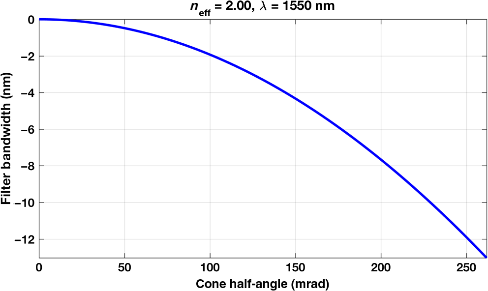
2.4.1.Calculation of background from solar fluxThe model described by McManamon et al.8 was used as a basis for our treatment of the solar background. In this paper, we assume a variable width filter that is adjusted based on the sensor field-of-view (FoV). The filter width can be as low as 1 nm, but, as the acceptance angle becomes larger, we need to increase the angular acceptance width of the filter. Spectral filter technologyCommercially available narrow-band filters can be placed in the receiver optical path to block unwanted background light. We assume that the narrowest achievable BW for a reasonable cost is for collimated light at normal incidence (for example, Alluxa offers a filter width of 0.7 nm for collimated light at ). As the sensor FoV is increased and rays at larger angles from the optical axis need to be accommodated, the range of effective wave vectors that must be accommodated widens; the wider filter BW passes more scene luminance, introducing more noise. The shift of the resonance wavelength with angle can be modeled as a Fabry–Perot resonator, as given in Eq. (2) and Fig. 4: Figure 4 indicates the required filter BW for typical material effective index . The widest sensor FoV occurs when a single array images the entire area; the angular distance to the corner of the array is where DAS is the angular subtense of a pixel and and are the number of pixels in each direction in the FPA. For and (the large DAS case), . Clearly, a wider filter BW, up to 9.3 nm, is needed, which will substantially increase background light. Recent developments suggest new filters that are much more tolerant to angle.Our comparison of detector technologies requires that the lidar can be operated in full sunlight. Table 3 gives the number of photons from the sun captured in each DAS per nanosecond, using a 1.0-nm wide filter. Background photon rates for wider spectral filters are obtained by linear scaling from this table. Table 4 then provides the number of background photons from the sun for specific cases of interest in this analysis. Table 3Number of photons captured per nanosecond in each detector for a 1.0-nm wide filter, with 1.55-μm wavelength.
Table 4Number of background photons from the sun for relevant cases.
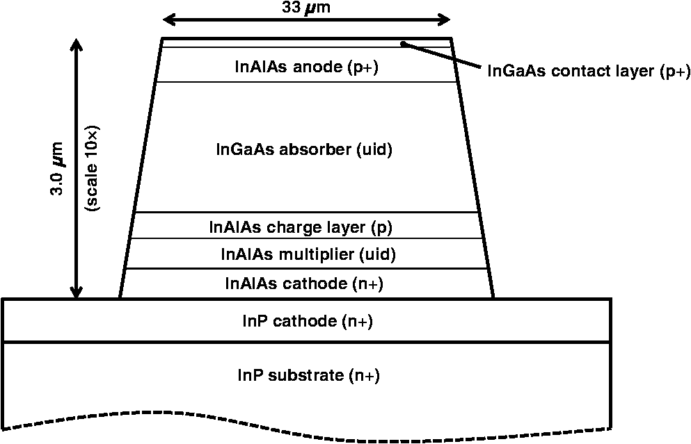
2.5.Link Budget Calculations to Determine the Required Laser Energy, Once the Required Number of Photons per Pixel is KnownFor each modality, we use the same link budget equations to determine how much energy per pulse we will need for the scenarios, based on how many photons reach each detector. A 2012 review9 article shows where is the received power, is the transmitted power, σ is the lidar cross-section, is the area illuminated, is the area of the receive aperture, is the transmission through the atmosphere between sensor and target, and is the optical system transmission efficiency. If we multiply both sides of Eq. (4) by a laser pulse width in units of time, this becomes energy received and transmitted. We can then solve for transmitted energy: whereFor 23-km visibility, is at 1550 nm.10 The required received energy, , can be specified as the energy in photons. We assume a wavelength of 1550 nm, for which We assume a system efficiency through the optical train of . We assume the area illuminated is 1.1 times as large as the angular area covered by our detectors to allow for some illumination inefficiency. This area grows with range. The cross-section is the reflectivity, , times the area seen by a given detector, which also grows with range: This is similar to Eq. (1), but with no foliage poke through, so the whole pixel is viewed. The ratio of area illuminated to cross-section is where is the number of detectors. Based on Eqs. (5–9), we can solve for required transmitter energy per pulse:For each modality, we can then calculate how much energy is required to map the area in each of the scenarios based on that detector’s required value of . The energy calculated by Eq. (10) is only for the number of pixels covered by a single detector array. For example, in the case of the GMAPD, we use a detector array. In our near-range scenario, the scene would be covered by stepping the GMAPD array’s FoV four times and the energy computed by Eq. (10) would be multiplied by a factor of 4; in our far-range scenario, we have , so the energy calculated by Eq. (10) would need to be multiplied by a factor of 256. For the near-range GMAPD case, if we use a smaller DAS to alleviate solar background, the number of required steps would increase commensurately. Multiple flash images of the same area of the scene may be required to collect geometry and/or grayscale data of the precision required by each scenario, depending on detector type. For example, GMAPD cameras are often designed to have low probability of detection per pulse, with the image built up by accumulation of multiple pulses against the target. The number of laser shots required per array step across the scene also multiplies the result of Eq. (10) when computing the total energy required by a given detector for a given range scenario and data product. 3.Calculations for InGaAs Geiger Mode Avalanche Photodiode CamerasLidar systems using arrays of GMAPDs were first proposed by Marino11,12 and demonstrated by MIT Lincoln Laboratory.13 Development work has continued to advance the technology for Geiger-mode ladar components, systems, data processing, and data exploitation in many research groups. Figure 5 shows a structure for a GMAPD detector.14 Our analysis relies on previous work by Fouche,15 who analyzed signal requirements in the presence of background noise. Recent modeling by Kim et al.16 provides a detailed description of example system behavior. We restrict our analysis to commercially available Geiger mode cameras. We consider commercial framing cameras with up to 186-kHz frame rate for the or up to 110 kHz for the format. An asynchronous readout is also now commercially available. This is capable of even higher readout rates limited only by the dead time between detections. In GMAPDs, the detector is biased above the breakdown voltage, so a photoelectron generated in the absorber region will result in a large avalanche, often resulting in a voltage fluctuation on the order of 1 V. If one photon, or many photons, hit the detector, the same large avalanche occurs. There is a dead time of 400 ns to after each triggered event, which can block detection of photons arriving later unless the probability of avalanche is kept low. For the case with foliage poke through, we set the average number of photons per pixel to be 0.8 photons returned for the expected range and reflectivity of the target or a 20% probability of detection per pulse given a PDE of 25%. With GMAPDs, there is crosstalk between detectors that is caused when a photon emitted during breakdown of one pixel triggers breakdown in another pixel. The noise due to crosstalk tends to be concentrated in the range region, where most of the detections occur. Even there, crosstalk noise is much smaller than noise due to background light for the cases analyzed in this paper. GMAPD flash imaging lidars tend to be designed to run at high frame rates, and many samples are used to capture the necessary number of photodetection events to achieve the signal level requirements. Laser pulse energy is lower, the number of photoelectrons generated per pulse is low, and the probability of a pixel firing is low. This has the technical benefit of keeping peak laser intensity low since each pulse is weak while maintaining high average power. This means that when we calculate required energy to 3-D image in a region, the main thing we vary will be the number of pulses, not the energy transmitted per pulse. Fig. 5Schematic illustration of a diffused-junction planar-geometry avalanche diode structure. The electric field profiles at right show that the peak field intensity is lower in the peripheral region of the diffused p-n junction than it is in the center of the device. 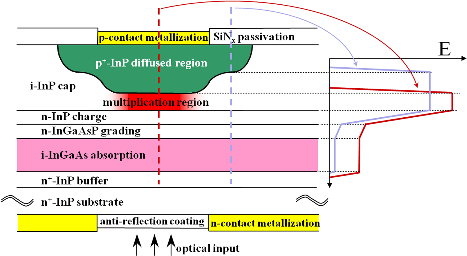 There are multiple detection events that can trigger a GMAPD receiver: the detection of a desired target photon, the detection of an undesired foreground clutter photon (such as backscatter from foliage), the detection of undesired background radiation (such as the sun), or the undesired detection of a dark electron. Cross talk can also trigger a GMAPD. If we send out many laser pulses, we will get coincident returns (returns in the same range bin) for reflection from a target or from fixed foreground objects, but returns from dark current, background, fog, snow, or rain will provide distributed returns with very low probability of range coincidence. 3.1.Effect of a Bright Sun Background on Geiger-Mode Avalanche PhotodiodesOne of the first things to address for GMAPDs is if background from the sun will affect either of the two scenarios. We conclude that it will not significantly affect the small DAS case but will significantly affect the large DAS case. Solar background is detrimental in two ways: blocking and noise, with blocking as the more important for this analysis. If the GMAPD undergoes an avalanche before the signal photons arrive, the detector is “blocked” and is unable to detect the signal until after the dead time. On the other hand, noise can cause the system to erroneously declare a surface to be present. Given a background photon rate per pixel of taken from Table 4, a PDE of 25%, and a gate width during which the APD is sensitive, the mean number of photoelectrons generated in the APD by the sun before the signal occurs is where is the speed of light and the factor of two accounts for the round trip. The Poisson distribution says that the probability of the APD not undergoing breakdown before the signal arrives (i.e., the probability of zero photo-electrons) is where is the probability of blocking. To keep the blocking loss below , the number of background photoelectrons must be kept belowFor a gate width , the background must be below . Clearly, DCRs, which are typically 1 to 10 kHz, can be neglected. The background photon rate can be limited by introducing attenuation on the receiver, reducing the aperture, or increasing the focal length and therefore reducing the pixel DAS. The GMAPD community prefers to increase the focal length while maintaining the aperture diameter to reduce blocking loss. The disadvantage of decreasing DAS instead of aperture diameter is that we then must scan more locations to develop the FoV required by the scenario. This will probably increase collection time. In line 2 of Table 5, we take values from line 2 of Table 3. We see in Table 3, line 2, that if we have a 25-mm diameter aperture and a DAS of 2.5 mrad, then we have . In Table 5, we see for that case the sun completely blocks our detector, showing 0% probability of not having an avalanche. This is the baseline case for our near-range, large DAS, scenario. From line 4 of Table 3, we have a gate width and . In that case, we will have a 70% probability of not being blocked if we either reduce our aperture diameter from 25 to 5 mm while keeping the DAS at 2.5 mrad or if we reduce the DAS to 0.5 mrad while maintaining a 25-mm diameter receive aperture. In either case, the result is the same in terms of sun blockage. For the gate width , we can either reduce the aperture size to 2.5 mm in diameter or the DAS to 0.25 mrad to avoid sun blocking. The smaller DAS case can use a narrower filter width, so that is one reason it will result in lower energy than decreasing the receive aperture size, and, of course, it provides higher resolution. Innovative processing will also provide a significant advantage for reducing the DAS compared to reducing the receive aperture diameter. In the next section, we will talk about coincidence processing, which is used by GMAPDs to achieve the required 90% probability of detection. If we reduce the DAS by a factor of 5 in each dimension, then each of our is made up of 25 . For surfaces that are smoothly varying, we can use these 25 samples to do coincidence processing, resulting in the need for as much as fewer pulses. This will reduce required energy for mapping the area. Table 5Probability of avalanche from background sun photons.
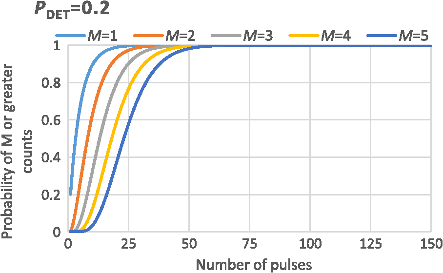
3.2.Coincidence Processing for DetectionWhen using GMAPDs in a foliage poke through scenario, we keep the probability of detection from a single pulse low because of the dead time after an avalanche (e.g., ). This preserves our ability to see objects farther in range then the initial return. Sometimes people use even lower probability of detection, such as 0.1. If we do not have mixed pixels with multiple range returns, we can allow the probability of detection to increase. For GMAPDs, we want to determine the number of pulses, , that must be transmitted to cause a GMAPD pixel to fire on pulses scattered from the surface of interest (we anticipate that M will be a minimum of two or three detections from the surface of interest). This coincidence detection will determine a real return from a physical object, as compared to a random false return. We rely on the fact the noise is randomly distributed in time, whereas returns from real objects only occur at the range of an object. We ignore nonuniform detector illumination and sensitivity. The probability of detecting a photon backscattered from the object of interest can be expressed as a conditional probability:17 where is the probability of detecting a photon backscattered by the object given that a photon scattered by some intervening obscurant (or dark count) has not been detected and is the probability of not detecting a photon from an intervening object. Since detecting a photon from an intervening obscurant is a binary event (it either is detected or it is not detected), the probability of not detecting a photon from an intervening obscurant is just one minus the probability of detecting that photon. Hence, Eq. (14) can be written as where is the probability of detecting a photon from an intervening obscurant or a dark count. As indicated earlier, the laser radar parameters can be adjusted so that the average values for and on a single pulse will be much less than 1. Multiple pulses will then be required to achieve high probabilities of detection. If the probability of detection is increased for the case with low reflectivity in the foreground, then fewer pulses will be required but more laser energy will be required per pulse. The probability of detecting a photon backscattered from the object of interest is also a binary event. Therefore, the probability of detecting a specified number of photons, , backscattered from the object of interest, out of pulses, can be described by the binomial distribution as follows:11The value for can be calculated once the parameters of the lidar system are specified. However, some insight can be obtained without considering a specific system configuration. To do this, we recast Eq. (15) in the following manner: where is the ratio , which is the ratio of the strength of scattering from the intervening obscuration and the strength of the return from the target of interest. In this form, a value for can be specified (controllable through the parameters of the laser radar imaging system) and the relative strength of backscatter between the intervening obscurants and the object can be treated as a parameter. As can be seen from Fig. 6, with a design probability per pulse of 0.2, nine pulses will provide two pulse coincidence with a 90% probability, and 14 pulses per detector should provide 90% probability of coincidence detection with three pulses. If we used an individual probability of 0.1, then this would be 38 and 52 pulses, respectively, and, with a probability of 0.15, we would need 25 pulses for two coincidences and 34 pulses for three coincidences. For a 0.04 probability, we would need 96 and 132 pulses. Obviously, more coincident pulses provide a higher probability that we are seeing a return from a hard target. Each avalanche resulting from scatter at a certain range will occur at a random location within the pulse width. One interesting result is the case of our large DAS scenario; we will reduce the DAS in both directions by a factor of 5 for bare earth and a factor of 10 for foliage poke through, resulting in 25 and 100 times as many samples. If we aggregate 25 small detects into one ground sample distance, GSD, then we can use a single pulse to obtain 15% probability of two pulse coincidence, and, in the case of aggregating 100 small area detections, we can go down to 4% probability of detection as a design criteria and still use only a single pulse.Since we desire maximizing the number of detections from the object of interest rather than the obscurations/false counts, we desire maximizing the value of given the constraint that , where is the ratio of near-range reflected light to target reflected light. As a reminder, is the probability of detecting a photon from the object of interest, whereas is the probability of detecting a photon from the object of interest with no obscuration. For our foliage poke through example, we have twice as much near-range reflections as we do target reflections, with the last return considered the target. In that case, . Two-thirds of the return flux come from the foreground surfaces and one-third from the final surface. We maximize the probability of detecting a photon from the object of interest by differentiating Eq. (17) with respect to and setting the derivative equal to zero. We find that the maximum value occurs for This can guide where we set our design probability of detection. With our case of for foliage poke through, we want a design of 0.25, or 1 photon received from the target with a 25% PDE, not much different than our case without foliage. We note that the expression for is valid for . Traditionally, when designing GMAPD lidars, people design with 0.1 to 0.2 probability of avalanche from the target or 0.4 to 0.8 photons with a PDE of 25%. To measure grayscale using GMAPD, multiple pulses are transmitted and the grayscale is built up one photodetection at a time. We compute the number of samples that must be transmitted to achieve the required number of photodetections. We use the term “samples,” because we can multiply the number of pulses times the samples per pulse to obtain the number of samples. The required number of photodetections is determined by the need to have the gray level separation large enough so that fluctuation in the number of detections is smaller than the gray level separation. Since the mean probability of detection on any given pulse is less than 1, there will be a fluctuation in the number of detections that will be obtained for a given number of transmitted pulses. As discussed above, the number of detections for a given number of transmitted pulses is a binomial distribution shown in Eq. (16). For a binomial distribution, the mean number of detections out of pulses is . The variance in the number of detections is (). To measure number of gray levels (), we need separations, each of which is 3.34 times the standard deviation. The factor of 3.34 is so that of the probability distribution is contained within the gray level separation. Hence, we need As specified earlier, we have assumed a variation in reflectivity from 0.05 to 0.15, or a 10% variation in reflectivity. Once and are specified, can be computed from Eq. (19). We can see in Eq. (19) that the required number of pulses is proportional to the square of the desired number of gray levels. For the small DAS case, we need to map an area of . With commercially available GMAPD cameras, we can either use a detector array or a detector array. Even with the array, we will need steps, or a total of 256 step stares for the small DAS scenario. For the large DAS case, we only need with a DAS of 2.5 mrad each, so we could take four steps using the format GMAPD array. If we reduce the DAS to reduce sun blocking loss (instead of decreasing aperture) than we need to increase the number of step stares. To fill the same area while reducing the DAS to will increase the required number of steps from 4 to 100; for the foliage poke through case with a DAS of , it increases the required number of steps to 400. The foliage poke through case has a larger window in range, so it requires more reduction in DAS to prevent detector blockage by the background from the sun. This small DAS will allow us to use a 1-nm wide filter, whereas with a large DAS, we would need to go to a wider wavelength filter. Also, the smaller DAS will increase angular resolution of the image and will reduce the required number of pulses because we can obtain more samples per pulse. In Table 6, we show the required number of samples, , and the required mapping energy for no grayscale and for either 3 bits, 8 gray levels or 6 bits, 64 levels of grayscale for the large DAS case. The number of pulses required for the no grayscale case is determined by how many pulses it takes to have a 90% probability of coincidence between two samples at the same range. In each case, we have chosen this to be one pulse because we are getting 25 or 100 samples from one pulse. We set the values to 25 or 100. The number of pulses required for grayscale comes from Eq. (17). is the case for no obscuration, where is our foliage poke through case with two times as much energy being reflected prior to hitting the final target. Table 6Required number of pulses and energy required for the large DAS case.
Next, we will look at the small DAS scenario. Table 7 shows the required total energy to map the small DAS case using GMAPDs. With grayscale, especially higher levels of grayscale, we see that the required energy is significant. Table 7Small DAS number of pulses and energy required.
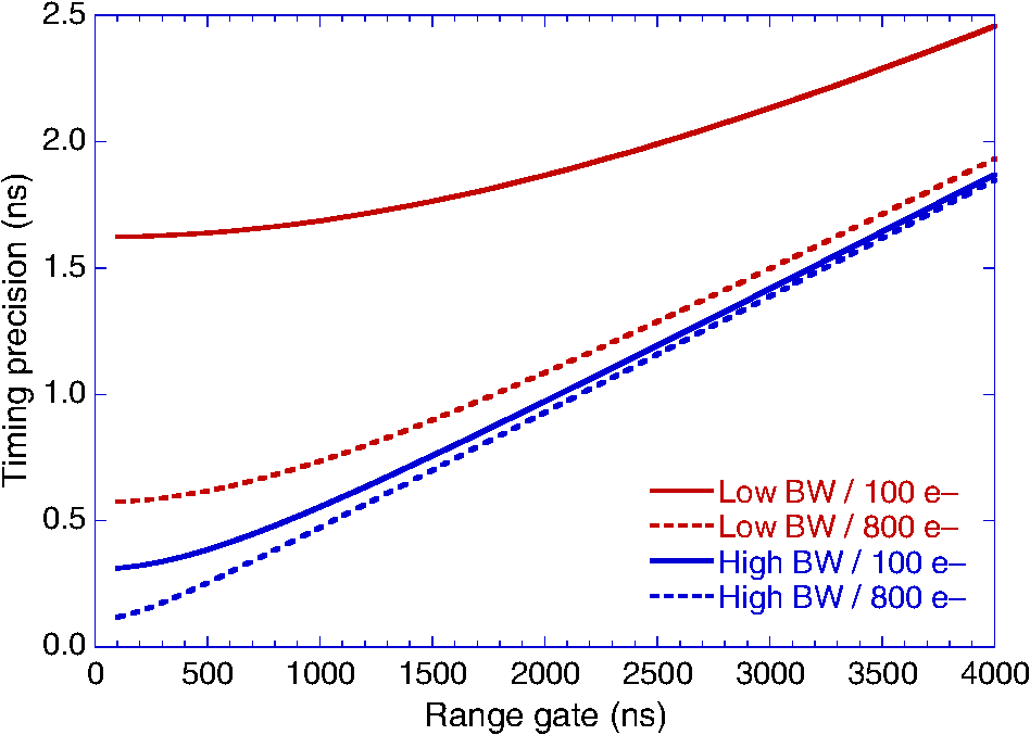
The range precision for these scenarios is not a challenge for GMAPDs and could be significantly better. This will be further discussed in the summary section. 4.Calculations of Required Energy for Linear Mode Avalanche Photodiode Cameras4.1.Calculations for InGaAs Linear Mode Avalanche Photodiode CamerasInGaAs LMAPDs are manufactured from thin films of and either or InP, epitaxially grown on InP substrates. The principal functional layers include the relatively narrow-bandgap (0.75 eV) InGaAs absorption layer and the relatively wide-bandgap multiplication layer made from either InAlAs (1.46 eV) or InP (1.35 eV), separated by a space charge layer, which ensures that the electric field strength in the absorber remains weak enough to avoid excessive tunnel leakage when the field in the multiplier is strong enough to drive a useful rate of impact ionization. This configuration is called the separate absorption, charge, and multiplication design. The layer ordering of absorber and multiplier relative to the anode and cathode—and the polarity of doping in the charge layer—depends on whether InAlAs or InP are selected as the multiplier material. Holes avalanche more readily in InP than electrons, so in an InP-multiplier APD, the absorber is placed next to the cathode and the charge layer is n-type; vice-versa for an InAlAs-multiplier APD. APD pixels may be formed either by patterned diffusion of the anode into the epitaxial material or by patterned etching of mesas from the thin film (in which case the anode layer was doped during epitaxial growth rather than diffused). Metal contact pads are deposited on individual pixel anodes, whereas a common cathode connection through the substrate is commonly used. In etched mesa designs, the pixel mesa sidewalls are chemically passivated and encapsulated to protect them from environmental degradation. Figure 7 depicts the structure of an InAlAs-multiplier, etched-mesa InGaAs LMAPD pixel of the type used in the detector array for which the calculations are made. Voxtel presently offers a prototype flash lidar camera with an InGaAs photodiode detector array that is TE cooled, and compatible LMAPD arrays are under development. Among others, advanced scientific concepts (ASC), Inc. Recently acquired by Continental, sells InGaAs LMAPD-based lidar cameras. The InGaAs LMAPD section is based on detector characteristics for Voxtel’s commercial InGaAs APD product, whereas detector characteristics for the HgCdTe LMAPD section are those published by DRS. In both sections, ROIC characteristics typical of two different design nodes—higher BW; higher circuit noise; smaller pixel format, and vice-versa—are used to analyze LMAPD FPA performance. In general, flash lidar ROICs designed to use linear-mode detectors employ a circuit in each pixel that includes a front end transimpedance amplifier to convert current or charge from the detector into a voltage signal, various filtering or pulse-shaping stages, and voltage sampling, storage, and readout circuitry. Two main sampling architectures are used: synchronous schemes in which the reflected waveform received by each pixel is regularly sampled with a period on the order of nanoseconds or asynchronous schemes in which a comparator is used to trigger sampling of reflected pulse amplitude and time-of-arrival when the signal exceeds an adjustable detection threshold. Provided the signal chain BW is high enough, both the synchronous “waveform recorder” sampling scheme and the asynchronous event-driven sampling scheme can support multihit lidar in which multiple reflections from a single transmitted laser pulse, arriving within nanoseconds of each other, are separately resolved and timed to penetrate obscurants like foliage. In both cases, sampling is active during a range gate in which target returns are expected, samples are stored locally in each pixel during the range gate, and the accumulated waveform or pulse return data is read out from the array in between laser pulses. Higher sample capacity drives ROIC pixel footprint because of the area required for storage capacitors. In general, the event-driven sampling architecture requires less space to implement because fewer samples must be stored to observe a given number of pulse returns per laser shot. The regularly sampled measurement approach has been called a full-waveform lidar for cases in which a large number of samples are stored. The sampling architecture analyzed here is the event-driven, asynchronous type, with an in-pixel storage capacity of up to three range and amplitude sample pairs. This matches the foliage poke through case analyzed here. Generic characteristics typical of this architecture are applied in the analysis. High BW operation of the signal chain in a flash lidar ROIC pixel generally requires high current draw during the range gate, and the sourcing and distribution of the supply current becomes more challenging as the array format grows. For this reason, we analyze two different configurations: high range precision (higher BW) operation in which pixel current draw limits the active format to about and operation of a larger () format array with reduced range precision (lower BW). Typical camera frame rates are in the 1 to 10 kHz range but depend on the array format, the number of samples stored and read out per pixel, and the number of output data channels operated in parallel. Aside from differing supply requirements, range precision, format, and frame rate, it should also be noted that operation of the pixel signal chain at different bandwidths will affect absolute sensitivity. Most of the relevant noise sources are wide-band, so, all else being equal, operation of the signal chain with higher BW means more in-band noise and lower sensitivity. However, the signal chain’s BW also affects sensitivity to laser pulses of different shape and duration since the overlap of an input pulse’s frequency spectrum with the ROIC’s transfer function will determine how efficiently the signal is amplified. Here, we will assume that the sensor is responding to 4-ns FWHM pulses in the calculations for the low-BW configuration and to 1-ns FWHM pulses for the high-BW configuration. As will shortly be established, the high-BW configuration will not be required for the large DAS scenario (which requires 25-cm range precision) since the range precision requirement can be met in a single laser shot using the larger-format low-BW configuration. However, the smaller active format high-range precision configuration may be of use for the small DAS scenario (5-cm range precision). If the low-BW configuration is used in the small DAS scenario, then range measurements from multiple laser shots must be averaged to reduce the standard error of the mean in a range below 5 cm. We will look at whether more laser shots per array step with fewer array steps (low-BW configuration) or fewer shots per array step with more array steps (high-BW configuration) require less energy to develop the required 3-D point cloud for the small DAS scenario. Multiple range measurements will reduce the standard error of the mean by the square root of the number of range measurements, such that the minimum number of range measurements () of timing standard deviation , which must be averaged to achieve a particular timing precision requirement is as follows: The variety of InGaAs LMAPD FPA analyzed here makes pulse return time estimates by sampling an analog voltage ramp that is distributed to all pixels in the array. Sampling of the ramp is triggered when the rising edge of a signal pulse from a detector pixel passes through an adjustable detection threshold. The threshold level must be optimized to extinguish false alarms arising from circuit noise in the ROIC convolved with the multiplied shot noise on the APD pixel’s dark current and background photocurrent. The ROIC’s fundamental timing uncertainty relates both to the voltage noise on the signal that triggers sampling of the ramp (jitter) and to the noise associated with reading the sampled voltage itself (resolution): where is a signal level at the ROIC pixel input in units of electrons, for which the jitter () is known, is the mean signal level for which the jitter is to be estimated, is the read noise on the analog time stamp, is the dynamic range of the time stamp, and is the range gate duration. Stronger signals transition through the comparator threshold faster, reducing jitter, and a faster ramp rate maps a given magnitude of read noise to a finer temporal resolution, giving rise to the timing precision characteristics calculated in Fig. 8 for typical ROIC timing characteristics. Figure 8 suggests that the low BW camera configuration will require multiple pulses to range with 5-cm precision. With a 500-ns armed period and a very weak signal return (100 e− after avalanche multiplication), the range precision is only about 24 cm. To obtain a standard error of the mean range measurement equal to 5 cm, we would need 25 pulses at this weak signal level. However, only four shots are required for signal returns. Even for low-BW operation, for the large DAS case, we would only need one pulse of to obtain 25-cm range precision. Note that the 500-ns range gate is similar to the armed times used for the GMAPDs (333 to 667 ns for 50 to 100 m).Each pulse return at a given optical signal level has some probability, , of exceeding the detection threshold. In the large DAS scenario, where the ROIC’s native timing precision is adequate to achieve the range precision requirement of 25 cm, is both the probability of detecting a target surface within a pixel’s instantaneous field-of-view (IFoV) and the probability of ranging to that surface with the required precision. However, in the small DAS scenario with the low-BW configuration, multiple range measurements must be averaged to achieve the range precision requirement of 5 cm. In that case, if total laser shots are transmitted, the probability of detecting enough pulse returns to achieve a standard error of the mean less than 5 cm is where is the number of laser shots successfully detected. It should be pointed out that Eq. (22) gives the probability of detecting enough pulse returns to achieve a particular standard error of the mean range, but, in general, seeing the target surface with less range precision is an easier problem requiring fewer laser shots and/or a weaker signal.Approximating the amplitude distribution of the signal into the pixel comparator as Gaussian, can be approximated as where is the probability that the sensor pixel is able to record a pulse return at the time it arrives, is the comparator threshold in units of electrons, and is the standard deviation of the signal into the comparator, also in units of electrons; like , and are quantities referred to the ROIC pixel input. The total noise is where is the standard deviation of the signal into the comparator in the absence of an optical signal return, is the mean gain of the APD pixel, and is the APD pixel’s excess noise factor. The excess noise factor for this type of APD (but not the HgCdTe LMAPDs described in the next section) obeys McIntyre’s formula [Eq. (25)].18 Table 8 then shows the excess noise factor for a InGaAs detector array:Table 8Excess noise factor.
Conceptually, is three separate noise terms added in quadrature—a purely circuit-related noise term and the multiplied shot noise of the APD’s dark current and CW background photocurrent. According to Table 3, a background photon arrival rate per pixel of up to per nm of filter BW is possible in the worst case (near target scenario; 2.5 mrad DAS; 25 mm aperture). Figure 4 estimates that the best filter width we can have in this case is 9.3 nm, so the background flux in the large DAS case will be . For a , InGaAs/InAlAs APD pixel with 80% QE and 70% fill factor, operated at a mean gain of , the worst case background photocurrent is about 1.6 nA. This is about an order of magnitude larger than the APD pixel’s 0°C dark current at this gain, of about 0.2 nA. Filter width is not a problem in the far target scenario, with 0.1 mrad DAS. Table 3 gives a background photon rate of about , corresponding to about 4 pA of photocurrent, which is negligible compared to the pixel dark current. The worst case optical background combined with the APD pixel’s 0°C, dark current together contribute about RMS of multiplied shot noise at the ROIC pixel input, whereas with negligible optical background, the multiplied shot noise of the APD pixel’s dark current alone is about under these conditions. In the low-BW configuration, responding to 4-ns FWHM laser pulses, an input-referred pixel circuit noise of about can reasonably be achieved. In the high-BW configuration, responding to 1-ns FWHM laser pulses, the ROIC’s circuit noise would roughly double. Consequently, in the low-BW configuration, the difference between the worst case solar background and negligible background is RMS versus . The high-BW configuration would not be applied to the large DAS case because of its smaller format and the relaxed range precision requirement of that scenario; in the small DAS case, the optical background is negligible, and RMS for the high-BW configuration. It should also be remarked that if the APD pixel is operated at lower gain, such as , the detector shot noise is smaller. We make calculations for APD pixel gains of , , , and to find an optimal operating point. The arming probability appearing in Eq. (23) depends on when in the range gate the target surface is located (), the pixel’s false alarm rate (FAR) at that detection threshold setting, and the sample capacity of the pixel (). Since false alarms in an LMAPD receiver circuit are independent stochastic events whose average rate of occurrence is given by the FAR, Poisson statistics apply, and the probability that at least one unused sample storage location is available at the time the return from the target surface is received is where is typical of what can fit into a small-pitch ROIC design. To reduce the number of model parameters, one can set equal to the range gate duration , which corresponds to the conservative case of a target surface at the very end of the range gate.Like , the FAR depends on the detection threshold (), but the standard Gaussian approximation for the noise distribution does not accurately model APD noise. Instead, the McIntyre-distributed19 noise of the APD must be explicitly convolved with the Gaussian-distributed noise of the ROIC to find the amplitude distribution of noise pulses into the pixel comparator: where is the amplitude distribution of the noise into the pixel comparator, is a Gaussian-like discrete distribution that characterizes the pixel circuit noise, and is the average of McIntyre distributions for the multiplied output of an APD given a certain number of primary input electrons, weighted by the probability that each quantity of primary electrons will result from dark current and background photocurrent generation processes as calculated by Poisson statistics. The convolution is best performed numerically. Figure 9 shows the convolutions calculated for mean APD gains of , 10, 15, and 20 for a InGaAs/InAlAs APD pixel in the large DAS case and compares the convolutions to Gaussian approximations having the same mean and variance. While correspondence is fairly close near the mean, tail divergence is a significant factor for FAR calculations owing to the need to set a detection threshold that extinguishes the great majority of false alarms. Following Rice,20 the FAR is found from a prefactor that depends on the pixel signal chain’s BW, , and the value of the convolution at the comparator threshold ():Fig. 9Example convolutions of multiplied APD dark current and background photocurrent shot noise with circuit noise, compared to Gaussian approximations having the same means and variances, for 25-mm aperture large DAS case. 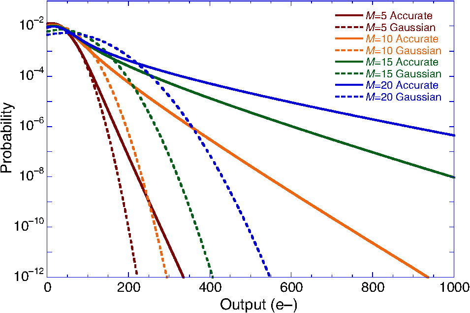 Fig. 10Probability of achieving 25-cm range precision in one laser shot, against bare earth (, dashed) and with two-return (, dotted) or three-return (, solid) foliage penetration, using LMAPD and the full format mode. 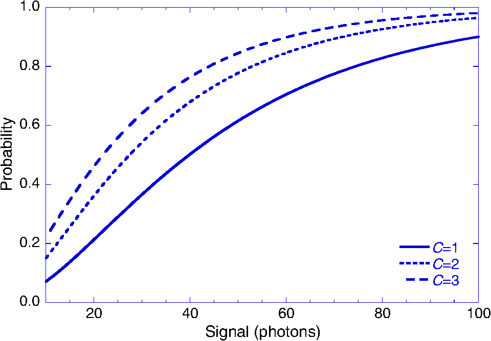 In addition to influencing the arming probability , the FAR also determines the probability of a false positive. In the large DAS case for which a single range measurement is required to achieve the specified range precision, Poisson statistics give the probability of at least one false positive occurring within the range gate of a given pixel as follows: In the small DAS case, where multiple pulse returns must be averaged to reduce the standard error of the mean range measurement, the coincidence of returns from the same range can be used to reject false alarms. If a validation rule of the form “ returns within of a given time-of-arrival” is applied, the probability of at least one false positive consisting of at least time-coincident false alarms occurring anywhere within the range gate, over total laser shots, is where the probability of at least false alarms out of laser shots occurring within any given time span is and the probability of at least one false alarm occurring within any given time span per shot is as follows:This is similar to the calculations we used for GMAPDs with a low probability of detection on a single pulse. To summarize, the probability of successfully measuring range to the required precision depends on the number of laser shots transmitted (), the number of range measurements required to achieve that precision (), and the per-shot detection probability (). The number of range measurements required depends on the signal strength (), as does the per-shot detection probability. also depends on the probability that the ROIC pixel’s sample capacity has not filled up with false alarms by the time a valid target return arrives, on the detection threshold (), and on the total noise (). The total noise includes a component that depends on the signal strength and a component that is present in the absence of the signal (). The analysis is completed by calculation of the FAR, which depends on and . For a given value of and , can be varied to maximize . The maximum value of is then compared to the critical value of required to achieve a particular probability of measuring range to the required precision (e.g., 90%), and is adjusted until the critical value is just barely reached. This determines the required signal strength at the ROIC pixel input. To translate into photons per pixel at the FPA (i.e., after collection by the camera aperture and any losses in the optical train), one divides by the product of the mean APD gain (e.g., ), the APD’s QE (80%), and the fill factor of the detector pixel (e.g., 70%). The radiometric model described in an earlier section is then used to backcalculate the transmitted laser pulse energy required to achieve the necessary signal level at the FPA under different scenarios (bare earth, foliage poke through, grayscale, etc.). Although multiple laser shots can be used for foliage poke through, as with a GMAPD, the very short (nanosecond) reset time of LMAPD pixels enables multihit lidar with a single laser shot if the ROIC can store multiple pulse returns. Figure 10 is a plot of the probability of achieving 25-cm range precision using an , , , LMAPD detector array operated at 0°C with the low-BW ROIC configuration. The optical background for the 2.5-mrad DAS (worst case) scenario was used. Curves corresponding to (single hit), (two-hit, single-shot foliage poke through) and (three-hit, single-shot foliage poke through) are plotted. The minimum signal level for which there is a 90% chance of ranging to 25-cm precision, against bare earth (), is 62 photons when the APD pixel operates at , 53 photons for , 56 photons for , and 61 photons for . The optimal gain is lower than the maximum gain in this scenario because of the strong background. Figure 11 is a plot of the probability of achieving 5-cm range precision in laser shots using an , , LMAPD detector array operated at 0°C with 70% optical coupling efficiency in combination with the low-BW configuration ROIC. Curves corresponding to (single hit; blue), (two-hit, single-shot foliage poke through; green) and (three-hit, single-shot foliage poke through; red) are plotted. The steps in the curves occur at signal levels, where the minimum number of range measurements that must be averaged to achieve the specified range precision, , changes by an integer, as calculated in Eq. (19). For example, the probability of detecting seven out of seven laser shots at a signal level of 39 photons is much lower than the probability of detecting six out of seven laser shots at a signal level of 40 photons, mainly because the number of required detections drops by 1 (as opposed to the marginally stronger signal return). That is why all three curves drop discontinuously between 39 and 40 photons. Fig. 11Probability of achieving 5-cm angle precision in seven laser shots, against bare earth (blue) and with two-return (green) or three-return (red) foliage penetration, using LMAPD and full format mode. 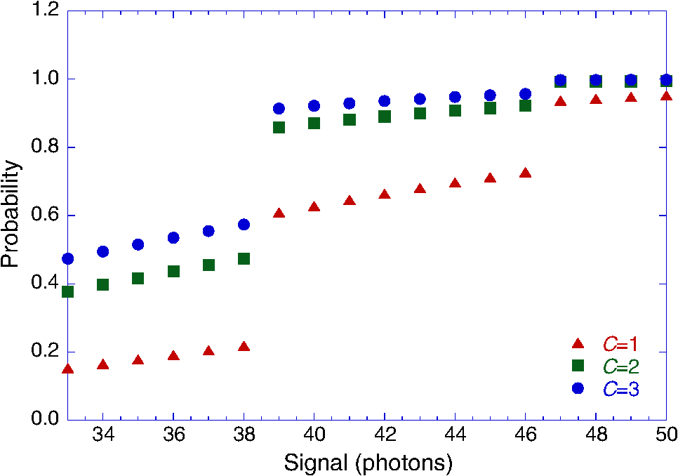 Figure 12 is a plot of the probability of achieving 5-cm range precision in a single laser shot using an , , LMAPD detector array with 70% optical coupling efficiency in combination with the high-BW configuration ROIC. Curves corresponding to (single hit), (two-hit, single-shot foliage poke through), and (three-hit, single-shot foliage poke through) are plotted. The difference in coverage between the high- and low-BW ROIC configurations should be considered when comparing this result to the low BW calculation of Fig. 9. Fig. 12Probability of achieving 5-cm range precision in one laser shot, against bare earth and with two-return or three-return foliage penetration, using LMAPD and a high-range precision mode. 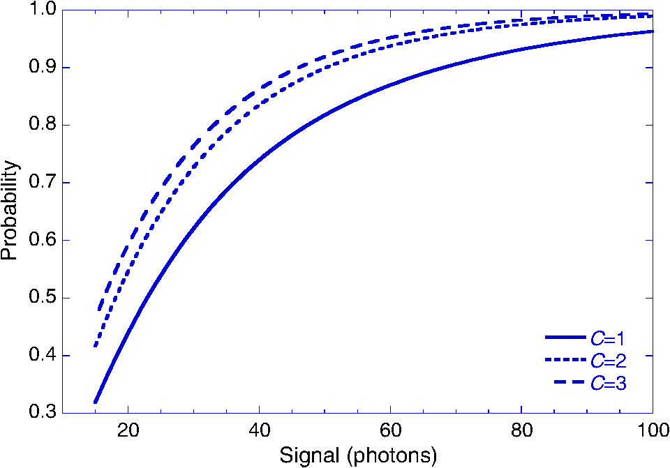 The number of laser shots and average signal return levels per shot required to have a 90% probability of ranging to the precisions specified for the near and far target scenarios are summarized in Table 9. Table 9Photons required per pixel and per shot for each of the cases.
The values in Table 9 are the required photons at the focal plane per laser shot and the number of laser shots, per pixel, per stepping of the FPA’s FoV across the scene. The figures given for foliage poke-through include the factor of reduction in cross-section for returns from the furthest obscured target surface and account for the higher detection threshold setting needed for multihit-per-shot lidar. In both the low BW, large DAS case and the high BW, small DAS case, a single laser shot is needed to achieve the specified range precision against bare earth and with foliage poke through. In the low BW, small DAS case, the least total energy is required when four laser shots are used against bare earth and three for foliage poke through. When total energy is calculated, the number of times the FPA’s FoV must be stepped to cover the scene will also be taken into account. Both high BW and low BW configurations are listed in Table 9, but, in the summary table of required energy for mapping, we only present data for the configuration that requires least total energy. ROICs of this architecture are also capable of grayscale range imaging if they are set up to sample and store the pulse return amplitude at the same time that they sample the analog time stamp. In passive imaging systems, the least-significant bit (LSB) of a sensor’s dynamic range is normally mapped to its noise floor, such that 6 bits of grayscale imaging would span the range from to the noise-equivalent input level. Passive imaging also assumes natural scene illumination. However, because the flash lidar architecture considered here uses an event-driven amplitude sampling scheme, pulse return amplitudes weaker than the comparator threshold will not be sampled. Furthermore, the ROIC’s amplifier chain is usually AC coupled, so natural continuous-wave (CW) scene illumination will not trigger sampling except through its contribution to the FAR. Grayscale imaging with such a ROIC is active imaging of the reflected laser pulse intensity. As such, the granularity of the grayscale image is still the noise-equivalent input level of the sensor, but the dynamic range spanned is offset from zero by the detection threshold. By the same token, the dynamic range available for grayscale imaging is smaller than the dynamic range of the signal chain into the threshold comparator. The grayscale resolution of a conventional passive imager is often expressed as a dynamic range in bits, which is calculated from the camera’s analog dynamic range by equating the LSB to the camera’s noise floor. However, optical signal shot noise increases as the square root of signal level, so an LSB, which represents the noise at zero signal (i.e., in the dark), does not quantify the accuracy with which nonzero signal amplitude can be measured, nor is it possible to define an LSB of a fixed size that exactly expresses signal amplitude measurement accuracy for all signal levels within an imager’s dynamic range. By contrast, this paper quantifies grayscale resolution based on there being a 90% probability that any given signal return amplitude measurement lies within a set interval centered on the average return level corresponding to the true target reflectance. The signal interval for which the calculation is made is that spanned by a reflectance bin of specified width. Equation (11) for the mean signal return level in photons per pixel can be rewritten as , where is a range-dependent function containing the radiometric aspects of the problem and is the target reflectance, which runs between and . If the range spanned by the target reflectance is divided into range bins, the reflectance bin width is . The mean signal range spanned by a reflectance bin is therefore which shows that a reflectance bin of a fixed size results in signal bins of variable size, dependent on . For instance, if , then photons for and for , etc.The bin width in photons increases linearly with mean signal strength, but the amplitude noise—given by Eq. (24)—includes a factor of the mean signal strength under the radical. This is the signal shot noise discussed earlier in connection to Fig. 2. For the scenarios analyzed here, signal shot noise dominates shot noise on background photocurrent and dark current, as well as ROIC noise, such that Eq. (24) can be accurately approximated as follows: For calculating the interval over which 90% of signal amplitude measurements will occur, the amplitude distribution in units of electrons that is sampled by the ROIC can be approximated as Gaussian, with the standard deviation () given by Eq. (34). With this approximation, 90% of signal return measurements will occur within of , or where is defined as the width in electrons of the interval centered on over which 90% of measurements will occur.Equation (35) allows one to solve for the interval in electrons, , given the mean signal per pixel in photons, , which is an input to Eq. (34) for the total noise. The interval in units of electrons represented by can be expressed in units of photons by dividing by a factor of , which is necessary to compare it to the signal span of a reflectance bin given by Eq. (33). The signal level required to achieve a specified grayscale resolution can be found by equating to from Eq. (33) and solving for the value of that satisfies the equality. However, the signal shot noise from Eq. (34) depends on rather than and varies from pixel to pixel because can vary from pixel to pixel depending on the average reflectance of the target scene within each pixel’s IFoV. To simplify the analysis, we make calculations using the average reflectance of . In that case, where is the function of APD gain given by Eq. (25) for InGaAs LMAPDs, also shown in Table 8, and is a fixed value of about for HgCdTe LMAPDs. For 6 bits of grayscale resolution, the specified reflectance span, and an effective QE of 56% (corresponding to 70% optical coupling efficiency and 80% detector QE), Eq. (36) gives ; for 3 bits of grayscale resolution with these parameters, . Recall that , so, for , the signal level per pixel required for the grayscale task is one-tenth the value of given by Eq. (36). For the InGaAs LM APD characterized by , , 3.52, 4,55, and 5.56 for , 10, 15, and 20, respectively, as shown in Table 8. Although operation of the APD at higher gain is beneficial from the standpoint of the 3-D imaging task, it results in worse grayscale imaging performance because of excess multiplication noise. This is a familiar result for LMAPDs, which are typically used in systems where signal shot noise is dominated by amplifier noise or where accurate measurement of signal amplitude is less important than discriminating signal pulses from noise.Equation (36) shows that the specified 6-bit grayscale resolution for is not practically achievable in a single laser shot, at low or moderate signal return levels, since the required signal level is on the order of . The requisite resolution is reached at for , 279,000 photons for , 360,000 photons for , and 440,000 photons for . For 3 bits of grayscale resolution, you can see a significant reduction in the required number of photons in Table 10. As we can see for the grayscale case, which is shot-noise limited, gain loses its appeal. With no gain, , we use the fewest number of photons. Note that the required number of photons per pixel in this grayscale case is not dependent on which scenario we chose, the large or small DAS case. The power required will be different for each scenario because of the other link budget considerations. The number of photons required in a grayscale case of LMAPDs also is not dependent on whether we are doing foliage poke through or not, except for the factor of 1.6 due to some of the photons being blocked from hitting the final reflector, which will be taken into account when we calculate energy. Table 10Required number of photons to achieve a certain grayscale level for an InGaAs camera.
If signal return amplitude measurements from laser shots are averaged, the standard error of the mean amplitude measurement will drop as , such that in the shot noise limit, the laser energy per shot can be cut by a factor of . However, evaluated in terms of the total number of photons required to perform the measurement, no advantage is gained by increasing the number of laser shots. Although this analysis shows that fine resolution of reflectance bins requires strong signals, one advantage of an LMAPD-based sensor is the ability to collect several bits of grayscale data per pixel in a single laser shot. LMAPDs could be useful in applications for which the accumulation of a large number of laser shots on the scene is not practical but target discrimination is aided by less accurate reflectance measurements than analyzed here. The total energy required to 3-D image in the cases we have picked depends on how many pixels we are imaging and how many laser shots are required. For the large DAS case, we need , which can be accomplished in a single pulse with the low BW configuration. The small DAS case will image , so it would require 16 steps of a FPA or 256 steps of a array. The total required steps would require rapid beam steering if the high BW configuration is required, but for our test cases, where we consider total energy required, we do not need to consider these practicalities. Table 11 shows the required energy to map each of the cases in both high- and low-BW configurations, although we do not bother to populate the high BW case for the large DAS scenario because, for the large DAS scenario, the high BW configuration will always require more energy. Also, for the grayscale case, it does not matter if we assume high BW or low, so we only populate the low BW case. We can see that the high BW configuration requires less energy for each of the small DAS cases, even though in the practical situation, the beam steering technology might limit its use. The format limitation assumed for the high BW case illustrates a real circuit design tradeoff, but not the limit of what is possible. It is not an inherent limitation of InGaAs LMAPDs. This should be kept in mind when considering this calculation. Also, in this calculation, we only considered single stage InGaAs APDs. Multiple stage APDs exist in this material system and have the potential to increase gain and lower noise. These considerations serve to highlight how complex this comparison space is. For current ROICs, we can see that obtaining the required range precision for the small DAS scenario was a driving parameter. It would have been an even stronger driver if we required more range precision. For the 6 bit grayscale case, a lot of energy is required. Even for the 3 bit case, significant energy is required. When such high energies are required, it is likely that dynamic range limitations, and energy per pulse requirements, will require multiple pulses to provide such high energy. Table 11Required energy for the InGaAs LMAPDs and the various scenarios.
4.2.Calculations for HgCdTe Linear Mode Avalanche Photodiode CamerasLinear mode HgCdTe electron injection APDs (e-APDs) have been demonstrated in APD arrays fabricated by DRS, Raytheon, CEA/Leti (France), Selex ES (United Kingdom), and others. They exhibit a deterministic gain process that results in an excess noise factor near 1 that is independent of gain. Gains up to 1900 with low dark current have been demonstrated in photon counting FPAs.21 The HgCdTe APDs cameras as large as for 3-D imaging and for gated 2-D imaging have been demonstrated. Current HgCdTe LMAPD FPAs have bandwidths of 100 MHz that are preamp BW or minority carrier diffusion time limited. However, the fundamental BW that is set by carrier transit times across the multiplication region is quite high. A BW of 600 MHz that was system RC time constant limited has been measured at an APD gain of 3500 (gain ).10 The modeled fundamental, carrier transit time limited, BW is greater than 10 GHz.22 Linear mode HgCdTe e-APDs as fabricated at DRS are front-side illuminated cylindrical p/n−/n+ HgCdTe homojunction photodiodes in the HDVIP® (HDVIP® stands for “high-density vertically integrated photodiode.”) configuration, as shown in Fig. 13. The architecture for the APD is the same architecture used for production, non-APD, FPAs. The cylindrical junction is created around a small hole (or via) in a thin passivated p-type HgCdTe membrane that is epoxied to a silicon readout. Metal is deposited in the via to form the contact from the n+ surface to the input pad on the silicon readout that is under the diode. The array is then anti-reflection coated. APD operation is achieved in this structure by increasing the reverse bias to create a high-field multiplication region on the n- side of the junction. The p-side of the junction becomes the absorption region for the APD. For typical unit cell geometries, the diffusion lengths of the holes and electrons are greater than the lateral dimensions of the n and p-regions. Thus, at low bias, both the n and p sides of the junction contribute to the photosignal, and the optical fill factor is the area outside the via, normalized to the unit cell area, which is equal to the pitch squared. (It is assumed that the unit cell is surrounded by other unit cells in a 2-D array configuration with a center-to-center spacing defined as the pitch.) At high bias, the fill factor is given by the ratio of area of the p absorption region to the pitch squared and is typically greater than 60% without a microlens. Microlens arrays have been developed for high systems that provide 100% fill factor. Many HgCdTe cameras in various formats have been delivered, but we are not aware of a HgCdTe APD camera available as a commercial product. While you certainly can buy large format flash imaging cameras from DRS or Raytheon, these will typically be custom single camera purchases, likely to cost on the order of $500K or even more, possibly associated with some development you specify. A cutoff HgCdTe APD FPA can be operated actively in any spectral region from about 360 nm in the UV out to . The MWIR cutoff HgCdTe APD FPAs need to be cooled to near 80 to 110 K, so that is a disadvantage compared to InGaAs GMAPDs and LMAPDs. The required HgCdTe detector biases, however, are conveniently and are compatible with current CMOS ROICs. Shorter wavelength cutoff HgCdTe APD FPAs have been demonstrated that operate at higher temperatures, and even in the thermal electric cooler temperature range, but these are less mature. Low noise long wave infrared cutoff HgCdTe APDs have also be demonstrated. Diffusion dark current is typically negligible compared to tunnel dark current and background photocurrent at 80 to 110 K in 4.2- to cutoff HgCdTe FPAs. The major source of dark current at the higher gains (higher APD biases) is a bias-dependent dark current that is thought to be due to indirect tunneling processes in the multiplication region. Because this dark current is generated in the multiplication region, it is likely not to be fully gained, and, indeed, noise measurements indicate this.23 A simplified manner of handling the dark current in the modeling is to use measured dark currents at the bias that achieve the required APD gain. This dark current is then divided by the gain to give a gain normalized dark current. A worst case, upper limit, dark current can be estimated at any intermediate gain by multiplying this gain normalized dark current by the gain. Gain normalized dark currents as low as 0.2 fA () have been measured on , photon counting APDs at a gain of 1100 to 1200, but, typically, the gain normalized dark current for photon-counting APDs is (). The grayscale calculations for HgCdTe are the same as for InGaAs, except when we are using gain, in which case we would have and we assume a QE of 65%. Since the excess noise does not change with gain, we can simplify the table of required photons, as shown in Table 12. As it turns out, gain does not help us with gray scale, so instead of the values shown in Table 12 for number of required photons, we will use the value for from Table 10 when we do energy calculations for HgCdTe arrays. Table 12Required number of photons for gray scale using HgCdTe.
Table 13Required photons per pixel for detection using a HgCdTe LMAPD.
The methodology and assumptions about representative ROIC parameters that are used to analyze the InGaAs LMAPD camera were applied to analyze the HgCdTe LMAPD camera. Although linear gains in the thousands have been demonstrated, we made calculations for , 100, 150, and 200 with . We restricted our analysis to this range because we found diminishing returns at higher gains and because the calculated signal levels were approaching the photon counting regime, which would require a different method of analysis. In the linear mode photon counting regime, the method of analysis must be modified because the photocurrent pulse shape output by the detector pixel is no longer determined by the envelope shape of the transmitted laser pulse but, rather, by the fundamental impulse response characteristic of the LMAPD pixel. Since the frequency spectrum of the photocurrent pulse affects ROIC sensitivity and timing characteristics, different ROIC parameters are required in the single photon signal regime. Also, different models of FAR and detection probability are warranted. We assumed laser pulse widths of 1 and 4 ns. The background photon arrival rate dominates the dark current by a wide margin in both scenarios. In the near target scenario with 2.5-mrad DAS, the background rate results in a pixel dark current of 15.6 nA when the pixel operates at ; the background rate results in 43.1 pA. In the large DAS case, a FAR model similar to Eq. (28) applies. However, in the small DAS case, the rate of background photon arrival is so low that false alarms are better modeled as the sum of a FAR computed from the ROIC circuit noise and a FAR calculated using Eq. (23) with to estimate the detection probability per primary photocarrier. In both cases, the HgCdTe APD’s output distribution is approximated as Gaussian, although, in reality, an LMAPD’s gain random variable cannot fluctuate below unity. With this simplifying assumption, the model gives the following values for the minimum average signal return level at the focal plane required to achieve the 90% probability of ranging to the precisions specified. The figures given for foliage poke through include the factor of reduction in cross-section for returns from the furthest obscured target surface and account for the higher detection threshold setting needed for multihit-per-shot lidar. In low-BW configuration, a lower signal level is required for the small DAS scenario than for the large DAS scenario, despite the more stringent range precision requirement, for two reasons. First, the high solar background in the large DAS has a significant impact on the sensor’s FAR. Second, the high linear gain of the HgCdTe APD provides the ROIC with a strong signal, which can be timed with lower jitter. Table 13 summarizes the required number of received photon per detector for the various cases. Then Table 14 summarizes the required energy using HgCdTe LMAPDs for the various cases. We see that HgCdTe LMAPDs do very well. Even these detectors do not do well for 6 bits of grayscale however. Table 14Energy required for HgCdTe LMAPDs.
5.Calculations for Optical Time-of-Flight, Flash LIDARLidar traditionally has focused most heavily on using a high BW time sensitive detector. An alternative is to use integrating sensor arrays with no time sensitivity and to modulate the received light in time, thereby mapping time onto intensity. The Air Force looked into this in the early, 90s before any high BW FPAs were available, with a concept at the time called laser imaging and ranging system.24–27 A diagram of a polarization-based concept to measure range resolution is provided in Fig. 14. Two companies, TetraVue and General Atomics, have pursued this form of 3-D imaging. The biggest benefit is that this form of imaging can leverage commercial high resolution CMOS and CCD for 2-D digital imaging at high resolution and high precision. These commercial FPAs are very capable in the visible and are developing in the near IR. These arrays do not have any gain, but, because of the maturity level, they have reduced noise and are relatively sensitive. The major need for gain is to compete against noise, so if we reduce noise we will not need as much gain. In this approach, an illumination pulse fills the scene and the camera lens focuses some part of the reflected signal onto the digital imager through a modulator. The single modulator modulates the entire optical field simultaneously, causing a change in transmitted light for each pixel of the integrating CMOS or CCD array as a function of when the light incident on that pixel passed through the modulator. A second array can be used to obtain the relative reflectivity of the surface so that the derived range is independent of surface reflectivity. In this way, the traditional problem of parallel precision time measurement (with GHz to 100 GHz effective bandwidths) becomes a parallel precision intensity measurement problem, which is what modern CCD and CMOS arrays do well. If two arrays are used, then it is critical to align the two arrays accurately because the ratio of intensity or corresponding pixels in the two arrays is used to measure range. Assuming accurate alignment between the two arrays, the range precision is determined by the range noise, which is related to the RMS uncertainty in the intensity measurement of each simple pixel. For this reason, grayscale measurements are inherent in this lidar modality. For high precision modalities, the fundamental noise limit is determined by the shot noise of the photon field. For longer range, lower precision modalities, the noise limit is the read noise of the sensor. Today, even consumer-grade visible CMOS imagers are achieving read noise levels , and some high-end CMOS sensors approach without external cooling. Since integration times can be short, dark noise is not relevant. The RMS range precision scales as follows: where is the range, is the number of pixels in the array, is the collecting aperture diameter, is the surface reflectivity, is the illuminator pulse energy, and is the range ambiguity interval. is a proportionality constant and is a constant equaling 1 for read noise dominated modalities and ½ for shot-noise dominated modalities.OToF has advantages such as access to megapixel and larger FPAs for high lateral resolution or high pixel count, simultaneous acquisition of high bit depth grayscale imagery, good performance with high contrast scenes () and objects, and mm-scale range precision can be achieved for certain high signal, small range window, scenarios. Low-cost imager sensor arrays and electronics are available for $100s or $1000s, especially in the visible and NIR, and no cooling is required for a 3-D camera system. However, OToF 3-D cameras do not detect multiple returns in a single pixel, so mixed pixels give only the average range. Also, the need to use an external modulator, such as a Pockels cell, can result in more complex optical designs. 3-D imaging system designs have been devised for each of the two test scenarios using an InGaAs imager with an assumed 80% QE at 1550 nm. However, since OToF makes use of high dynamic range grayscale images, only the grayscale subcases are relevant. For example, in cases where the brightest objects (e.g., a 100% reflective surface in the same scene as the 10% reflective surface) fill the pixel well-depth, a 12-bit grayscale image can be obtained using commonplace 12-bit 2-D imagers. This availability of high dynamic range sensors also means that scenes with high contrast (even or ) do not affect the measurement. Range precision is better for the brighter areas than the nominal 10% reflectivity, scaling by the equation above. Solar flux is managed, particularly in the SWIR band, with short shutter times and small pixels, so any solar background has no effect on range precision. For the large range windows of 50 and 100 m, the range will have ambiguities as waveform repeats, as illustrated in Fig. 14. High range precision can be obtained, however, by repeating the sawtooth ramps. If we have 512 (9 bits) of intensity measurements, then we can have range resolution with a 50-m ramp and 20-cm range precision with a 100-m ramp. A second Pockels cell and sensor combination in the 3-D camera with a longer waveform can be used to remove ambiguities at the expense of additional complexity. 6 bits intensity measurement accuracy would allow less range resolution for a given ramp length. Grayscale imagery is intrinsic to OToF because of its single pulse acquisition. The actual available bit depth of these grayscale images for each scenario is determined by the ratio of a 100% reflective surface over the dominant noise term (read or shot noise) after binning and some image processing. The actual well depth of the pixel will be larger than this (which is useful for scenes where the relative range separation is large). For the large DAS scenario, the effective grayscale dynamic range is 7.4 bits. For the small DAS scenario, the effective grayscale is larger at 9.7 bits (12+ bit sensors are typically used). However, to get the 0.156% mentioned above to get 6 bits of grayscale intensity values from 5% reflective to 15% reflective surfaces, the noise equivalent input level is too high for the large DAS case. Therefore, the energy required has to be increased by for the bare earth case, which simultaneously improves the range precision to 7 cm. In the large DAS case with foliage, the higher relative precision required to cover the larger 15-m range distribution means that a smaller energy increase is required to exceed the noise equivalent input level (). For the small DAS case, the energy required to achieve the 5-cm range precision is sufficient so that the noise equivalent input is smaller than the 0.156% LSB for the grayscale. For near-range, large DAS, the equivalent pixel size for a 0.5-m GSD with an 18-deg FoV is for our OToF design. Such a large pixel would require a custom sensor with very large pixels. It should be better design to use a smaller pixel, e.g., () or similar, and to bin the pixels to achieve the format required for the target DAS. Binning also decreases the effective noise per metapixel, and there are designs that can bin before the readout to further reduce the effective read noise. We have assumed row- or columnwise binning before read-out. The information could be acquired in either a single frame ( format) or as a series of narrow aspect ratio images ( format) that are synchronized to the aircraft motion ( at flight speed). The total energy required to achieve the case 1 performance with a 5-m ambiguity interval is 1.1 mJ. The energy required does not change based on single frame or push broom capture. This corresponds to through the collecting aperture. However, the LSB is such that there are only 4 bits of grayscale in the image. For 6-bit grayscale image from 5% to 15% reflective surfaces, the required energy per pixel increases to 5.3 mJ. The resultant range precision in this case is 7-cm range precision. For the small DAS case with 0.1-m GSD, the equivalent pixel size with a 5.9-deg FoV is . This pixel size is close to typical pixel designs, and the area could be covered using a array in a single frame. The higher range precision requires substantially more energy, and this scenario is dominated by shot noise rather than sensor noise. The grayscale bit-depth of between 5% and 15% exceeds the 6-bit requirement without energy adjustment. The information could be acquired in either a single frame ( format) or as a series of 16 narrow aspect ratio ( format) images that are synchronized to the aircraft motion ( at flight speed). OToF lidar takes advantage of standard noise reduction techniques, which have not been taken into account using the LMAPD sensing modalities. 6.SummaryTable 16 summarizes the required energy for various imaging modalities. For the case of the InGaAs LMAPDs, we carried two BW settings but, for the summary, only used the BW setting that required lower energy. Table 15Energy summary OToF lidar.
Table 16Summary of energy required for various scenarios and cameras.
GMAPD cameras operate with a low probability of return on a single pulse but require coincident returns from the same range. GMAPD cameras require low energy per pulse lasers with a higher repetition rate. We see that the GMAPD cameras do well in both scenarios when doing bare earth 3-D mapping and 3-D imaging through trees. The large DAS scenario does not create a significant energy use issue because it uses many coincident samples from a metapixel. In grayscale situations, the GMAPD cameras do use somewhat more energy. Advantages of the GMAPDs are: (1) they are TE cooled; (2) they use low energy per pulse, high repetition rate lasers, which are easier to obtain because laser diodes are CW and because of damage thresholds of fiber lasers; (3) they can passively image in the near IR; (4) they have little noise, so their performance can be easily predicted; (5) these cameras are commercially available from at least two sources, Princeton Lightwave and Boeing Spectra-lab, and are moderately priced; and (6) the readout circuits are very simple. Disadvantages of GMAPDs are: (1) there is a dead time of 400 ns to after an avalanche. The probability of avalanche must be kept low, or we can only see a single range in a pixel with more than one return in range; (2) due to this blocking issue, high background, sun as a bright sun, can be an issue, requiring smaller apertures or increased resolution, but the innovative processing associated with using multisamples in a megapixel has mostly mitigated this; (3) forming the image requires significant processing due to both coincident processing and removal of motion; and (4) dynamic range is narrow to have the right number of return photons. The advantages of InGaAs LMAPDs are: (1) they are TE cooled; (2) they are commercially available from at least two sources, Voxtel and ASC; (3) they are moderately priced; (4) 3-D images can be formed on a single pulse; (5) 3-D images can be formed quickly and with simple processing. Disadvantages of the InGaAs LMAPD cameras are: (1) gain is relatively low, from 5 on up, due to excess noise and breakdown issues; (2) a complex ROIC is required; (3) because gain is relatively low, it is necessary to keep track of all noise sources; and (4) we need a relatively high energy per pulse laser. HgCdTe LMAPDs have , meaning essentially all the carriers generated during an avalanche are electrons. This allows very high gains, so these cameras are very sensitive while retaining linear gain. They require very low energy for mapping in many of the cases in Table 15. Other advantages are: (1) 3-D images can be formed on a single pulse, (2) 3-D images can be formed quickly and with simple processing; and (3) they can image passive and active from visible through the mid IR. A day/night passive imager can be inherently cobore sighted with an active imager. Disadvantages include: (1) these cameras are not commercially available, even though you can buy them from DRS, Raytheon, or possibly others, so they are more expensive at this time; (2) HgCdTe cameras need to be cooled to near 100 K, so they require a coke can size cooler; (3) these cameras require a complex ROIC; and (4) these cameras require high energy per pulse lasers. OToF using low BW cameras with a medium BW Pockels cell has the advantage of using commercially available 2-D cameras for flash 3-D imagery. In the visible or NIR you can obtain huge format cameras with tens of megapixels for hundreds of dollars, promising high performance at low cost. Even in the SWIR, you can obtain up to a custom camera, and smaller cameras for as low as $25K from multiple vendors. These cameras are mature and can have low noise uncooled, so, even though they do not have gain, they can be relatively sensitive while giving high dynamic range. The main disadvantages are that you need a Pockels cell and its cost. A secondary disadvantage is if you use two cameras, you must align them carefully. The OToF cameras show low energy use for 3-D mapping with grayscale. That said, it is likely that some of the other sensing modalities will be able to adopt some of the noise reduction techniques being employed. The OToF camera has the advantage of using cameras built for a large commercial market. If you want high range resolution, you are currently best off using either a GMAPD array or an OToF imager. HgCdTe arrays are probably second in BW/range resolution at this time. All LMAPD cameras have similar challenges in high range resolution. The range precision for these scenarios is not a challenge for GMAPDs and could be significantly better. GMAPDs typically have an advantage over LMAPDs in terms of inherent timing precision when detecting isolated optical pulses because the current pulses generated by breakdown of a GMAPD pixel are stronger, and are of much more uniform amplitude, than the current pulses emitted by an LMAPD pixel in response to weak signals. The mean response of an LMAPD pixel to an ensemble of identically prepared input optical pulses is proportional to the optical signal strength, which enables direct measurement of signal amplitude. However, an LMAPD’s response to such an ensemble of identical input signals varies stochastically around the mean, limiting the accuracy of a single amplitude measurement and affecting the timing of when the signal crosses the detection threshold of a decision circuit. When using LMAPD pixels, timing jitter is large if the APD’s response barely exceeds the detection threshold; range precision improves for stronger signal returns. Consequently, scenarios that prioritize the best range precision with the least transmitted energy tend to favor GMAPD detectors, whereas scenarios that require penetrating obscurants or collecting reflectance information in a single observation (for instance, to “freeze” a dynamic scene) tend to favor LMAPDs. In this paper, we have attempted to select scenarios that straddle these respective areas of strength and weakness, but these general characteristics should be borne in mind when considering specific applications. ReferencesM. A. Itzler et al.,
“Geiger-mode APD single-photon cameras for 3D laser radar imaging,”
in IEEE Aerospace Conf.,
(2014). http://dx.doi.org/10.1109/AERO.2014.6836476 Google Scholar
G. M. Williams et al.,
“Multi-gain-stage InGaAs avalanche photodiode with enhanced gain and reduced excess noise,”
IEEE J. Electron Devices Soc., 1
(2), 54
–65
(2013). http://dx.doi.org/10.1109/JEDS.2013.2258072 Google Scholar
M. Ren et al.,
“AlInAsSb separate absorption, charge, and multiplication avalanche photodiodes,”
Appl. Phys. Lett., 108 191108
(2016). http://dx.doi.org/10.1063/1.4949335 APPLAB 0003-6951 Google Scholar
S. J. Maddox et al.,
“Enhanced low-noise gain from InAs avalanche photodiodes with reduced dark current and background doping,”
Appl. Phys. Lett., 101 151124
(2012). http://dx.doi.org/10.1063/1.4757424 APPLAB 0003-6951 Google Scholar
P. F. McManamon et al., Laser Radar: Progress and Opportunities in Active Electro-Optical Sensing, 310 National Academies Press, Washington, D. C.
(2014). Google Scholar
M. J. Halmos et al.,
“Photon counting ladar,”
http://sti.usra.edu/clrc2011/presentations/Session%204/Summary%20M%20Halmos.pdf Google Scholar
P. Gatt and S. W. Henderson,
“Laser radar detection statistics: a comparison of coherent and direct detection receivers,”
Proc. SPIE, 4377 251
–262
(2001). http://dx.doi.org/10.1117/12.440113 PSISDG 0277-786X Google Scholar
P. F. McManamon et al.,
“A comparison flash lidar detector options,”
Proc. SPIE, 9832 983202
(2016). http://dx.doi.org/10.1117/12.2229068 PSISDG 0277-786X Google Scholar
P. F. McManamon,
“Review of ladar: a historic, yet emerging, sensor technology with rich phenomenology,”
Opt. Eng., 51
(6), 060901
(2012). http://dx.doi.org/10.1117/1.OE.51.6.060901 Google Scholar
I. I. Kim, B. McArthur and E. Korevaar,
“Comparison of laser beam propagation at 785 nm and 1550 nm in fog and haze for optical wireless communications,”
Proc. SPIE, 4214 26
–37
(2001). http://dx.doi.org/10.1117/12.417512 PSISDG 0277-786X Google Scholar
M. B. R. Marino and R. Spitzberg,
“A photon counting 3-D imaging laser radar for advanced discriminating interceptor seekers,”
in 2nd Annual AIAA SDlO Interceptor Technology Conf.,
(1993). Google Scholar
R. Heinrichs et al.,
“Three-dimensional laser radar with APD arrays,”
Proc. SPIE, 4377 106
–117
(2001). http://dx.doi.org/10.1117/12.440098 PSISDG 0277-786X Google Scholar
M A. Itzlera et al.,
“Advances in InGaAsP-based avalanche diode single photon detectors,”
J. Mod. Opt., 58
(3–4), 174
–200
(2011). http://dx.doi.org/10.1080/09500340.2010.547262 JMOPEW 0950-0340 Google Scholar
D. G. Fouche,
“Detection and false-alarm probabilities for laser radars that use Geiger-mode detectors,”
Appl. Opt., 42
(27), 5388
–5398
(2003). http://dx.doi.org/10.1364/AO.42.005388 APOPAI 0003-6935 Google Scholar
S. Kim, I. Lee and Y. J. Kwon,
“Simulation of a Geiger-mode imaging ladar system for performance assessment,”
Sensors, 13
(7), 8461
–8489
(2013). http://dx.doi.org/10.3390/s130708461 SNSRES 0746-9462 Google Scholar
E. A. Watson,
“New imaging modalities for laser-based systems,”
in IEEE Aerospace Conf.,
(2001). http://dx.doi.org/10.1109/AERO.2001.931391 Google Scholar
R. J. McIntyre,
“Multiplication noise in uniform avalanche photodiodes,”
IEEE Trans. Electron Devices, ED-13
(1), 164
–168
(1966). http://dx.doi.org/10.1109/T-ED.1966.15651 IETDAI 0018-9383 Google Scholar
R. J. McIntyre,
“The Distribution of gains in uniformly multiplying avalanche photodiodes: theory,”
IEEE Trans. Electron Devices, 19
(6), 703
–713
(1972). http://dx.doi.org/10.1109/T-ED.1972.17485 IETDAI 0018-9383 Google Scholar
S. O. Rice,
“Mathematical analysis of random noise,”
Bell Syst. Tech. J., 23
(3), 282
–332
(1944). http://dx.doi.org/10.1002/bltj.1944.23.issue-3 BSTJAN 0005-8580 Google Scholar
W. Sullivan et al.,
“Linear mode photon counting from visible To MWIR with HgCdTe avalanche photodiode focal plane arrays,”
Proc. SPIE, 9492 94920T
(2015). http://dx.doi.org/10.1117/12.2180394 PSISDG 0277-786X Google Scholar
G. Perrais et al.,
“Study of the transit-time limitations of the impulse response in mid-wave infrared HgCdTe avalanche photodiodes,”
J. Electron. Mater., 38 1790
–1799
(2009). http://dx.doi.org/10.1007/s11664-009-0802-7 JECMA5 0361-5235 Google Scholar
J. Beck et al.,
“Performance and modeling of the MWIR HgCdTe e-APD,”
J. Electron. Mater., 38 1579
–1592
(2009). http://dx.doi.org/10.1007/s11664-009-0684-8 Google Scholar
K. W. Ayer et al.,
“Laser imaging and ranging system (LIMARS): a proof of concept experiment,”
Proc. SPIE, 1633 54
–62
(1992). http://dx.doi.org/10.1117/12.59206 PSISDG 0277-786X Google Scholar
BiographyPaul F. McManamon is the president of Exciting Technology and Technical Director LOCI, University of Dayton. He chaired the laser radar study for the National Academy of Sciences and cochaired the Optics and Photonics study. He is a fellow of SPIE, IEEE, OSA, AFRL, DEPs, MSS, and AIAA. He was the president of SPIE in 2006. Until May 2008, he was a chief scientist, AFRL sensors directorate. He received the Meritorious Presidential Rank Award in 2006. Paul Banks is the founder and CEO of TetraVue, working to commercialize high resolution 3-D imaging for smart robotic vision. He received his PhD in applied physics from the University of California, Davis. His career includes work at Lawrence Livermore National Laboratory, and he was cofounder of a new Photonics Division at General Atomics. He has contributed in many areas of laser technology and applications, from ultrafast to directed energy. Jeffrey Beck received his master’s in EE from M.I.T. (Cambridge, Massachusetts) in 1972. He joined Texas Instruments in 1978 and was elected a distinguished member of technical staff in 1996. In 2004, he received the Military Sensing Symposium (MSS) Herschel Award for his discovery of the noiseless gain HgCdTe APD. He was elected MSS Fellow in 2006. He won the 2009 Innovation Award from Finmeccanica S.p.A, Italy. He is a staff scientist at DRS Technologies. Dale G. Fried earned his PhD in atomic physics in 1999 from MIT for the experimental realization of Bose-Einstein condensation in atomic hydrogen. He developed integrated optical waveguide devices for telecom applications at Clarendon Photonics until joining MIT Lincoln Laboratory in 2004. He played leadership roles developing prototype airborne Geiger-mode ladar systems for wide-area mapping and foliage poke-through applications. He founded 3DEO in 2014 to bring Geiger-mode ladar into widespread application. He holds seven granted patents. Andrew S. Huntington has led SWIR detector development at Voxtel Inc. since 2004, specializing in avalanche photodiode (APD) design and application of APDs to scientific and military sensing. His work at Voxtel has included computational modeling of impact ionization statistics to engineer lower noise multipliers for InGaAs APDs, APD epitaxial layer design, APD wafer fabrication process design, and performance modeling of sensor systems based on APD photo-receivers and focal plane arrays (FPAs). Edward A. Watson is a distinguished researcher of sensor technologies for the University of Dayton Research Institute. He is also a chief executive of Vista Applied Optics, an optical consulting firm. He retired in 2012 from the Air Force Research Laboratory after 30 years. His research interests include lidar, optical phased array technology, and novel remote sensing, such as low light level imaging and speckle characterization. He is a fellow of OSA, SPIE, and MSS and is an AFRL fellow. |
||||||||||||||||||||||||||||||||||||||||||||||||||||||||||||||||||||||||||||||||||||||||||||||||||||||||||||||||||||||||||||||||||||||||||||||||||||||||||||||||||||||||||||||||||||||||||||||||||||||||||||||||||||||||||||||||||||||||||||||||||||||||||||||||||||||||||||||||||||||||||||||||||||||||||||||||||||||||||||||||||||||||||||||||||||||||||||||||||||||||||||||||||||||||||||||||||||||||||||||||||||||||||||||||||||||||||||||||||||||||||||||||||||||||||||||||||||||||||||||||||||||||||||||||||||||||||||||||||||||||||||||||||||||||||||||||||||||||||||||||||||||||||||||||||||||||||||||||||||||||||||||||||||||||||||||||||||||||||||||||||||||||||||||||||||||||||||||||||||||||||||||||||||||||||||||||||||||||||||||||||||||||