Optical performance of piezoelectrically actuated MEMS tunable lenses with various pupil geometries

Mahmoud A. Farghaly; Muhammad Nadeem Akram; Einar Halvorsen

doi:10.1117/1.OE.56.3.035104

21 March 2017 Optical performance of piezoelectrically actuated MEMS tunable lenses with various pupil geometries

Mahmoud A. Farghaly, Muhammad Nadeem Akram, Einar Halvorsen

Author Affiliations +

Optical Engineering, Vol. 56, Issue 3, 035104 (March 2017). https://doi.org/10.1117/1.OE.56.3.035104

Abstract

A square geometry for the diaphragm of microelectromechanical systems (MEMS) tunable lenses with circular pupils is often used. This square diaphragm introduces aberrations that would not be present for a circular diaphragm and the question arises of whether it could be advantageous to also consider other than circular geometries for the pupil. To investigate this question, we have extended a previously established modeling framework for piezoelectrically actuated MEMS tunable lenses to devices with general polygonal-shaped pupils. It models the static optoelectromechanical coupling for symmetric configurations based on laminated-plate theory, linear piezoelectricity, and ray tracing. The framework helps to find geometrical parameters that give a diffraction-limited tunable lens with a minimum F-number. The tunable lens’ optical performance and its focusing capability, alone and in combination with a fixed lens, were calculated in terms of object distances and actuation voltages. Using the modeling framework, we show that the modulation transfer function of the tunable lens and the fixed lens combination remains the same up to a ±10-deg field of view after voltage adjustment to refocus on near objects. In addition, we found that pupil masking of the tunable lens can provide a beneficial tradeoff between the lens dioptric power and its RMS wavefront error.

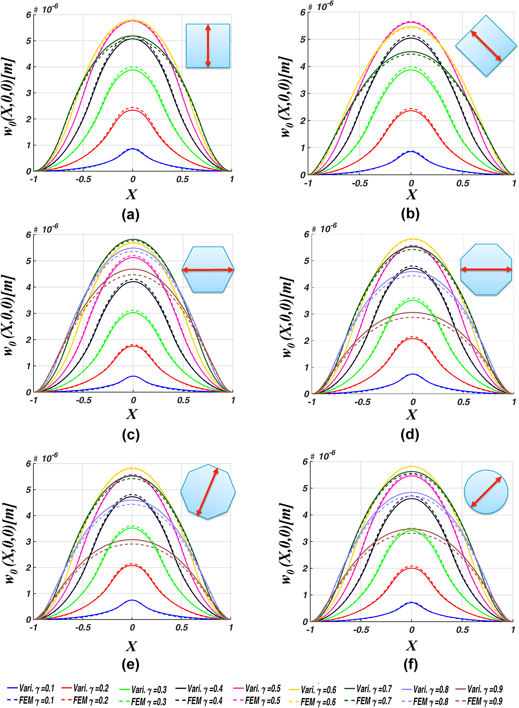
1. Introduction

An autofocus mechanism, which allows image capturing with sharp details, has become an essential feature in mobile-device cameras. The conventional macroscale technologies, such as voice-coil motors¹ and ultrasonic motors,² are currently used to tune the focus in commercial lens systems. Nevertheless, microelectromechanical systems-(MEMS)-based tunable focus lenses are recently trending in providing low-power microscale solutions with faster scanning rates over the focusing range.³^–⁸ MEMS autofocus lenses have no sliding parts within the camera housing, consume less power during focus adjustment, and cause no loss in the field of view, as compared to the conventional technologies.

The microscale technologies provide two ways to tune focus through modifying either the medium’s effective refractive index or the interface slope between two refractive media. Liquid crystal lenses use a controllable electric field to reorient liquid-crystal molecules to create a spatially varying refractive index that converges or diverges the light rays.³ Tunable microfluidic lenses⁴^,⁵ control pressure in a liquid trapped in a fluidic cavity to deform the cavity’s top surface. One tunable liquid lens uses the electrowetting phenomena to make the interface between two polar liquids convex or concave.⁶ Piezoelectrically actuated lenses deform a transparent membrane between two refractive media. These media can be air and a fluid,⁷ or air and a polymer as in the TLens case.⁸

The aforementioned tunable lenses can be a unit lens in tunable-focus microlens arrays.⁹ These arrays are multifocus systems that provide depth sense needed for space perception in 3-D imaging systems.¹⁰ Moreover, they practically grant real-time image acquisition in coherent anti-Stokes Raman scattering spectroscopy.¹¹ Each unit cell could have different pupil geometries, such as a circle,⁴ a hexagon,¹² or a square.¹³ A unit lens’ pupil shape affects the resolution of the reconstructed object done by integral photography.¹⁴

In this article, we focus our attention on the optical performance of piezoelectrically actuated MEMS tunable lenses with differently shaped pupils. We use a modeling framework to predict their static optoelectromechanical performance. The first part of this framework is to model the static electromechanical performance based on variational methods introduced in a previous work.¹⁵ For verification of the electromechanical model, we compare the lens displacement from the variational solutions against the finite element method (FEM). The The second part is to quantitatively investigate the tunable lens’s optical performance using ray tracing by analyzing its $F$ -number ( $F #$ ), RMS wavefront error (RMSWFE), and modulation transfer function (MTF). The MTF response of the tunable lens in combination with a fixed lens¹⁶ remains essentially the same for a ±10-deg field-of-view (FOV) when the object is located at different distances after actuation voltage adjustment. Beyond that FOV, the MTF response is degraded due to the tunable lens’ off-axis aberrations. In addition, we have explored pupil masking for actuators with different pupil geometries and found that it provides tradeoffs between the lens dioptric power $1 / f$ and RMSWFE for a 45-deg rotated square pupil, especially with larger aperture areas.

2. Principle of Operation

The MEMS tunable lenses that we study here bend a transparent diaphragm by piezoelectric actuation to modify the interface slope between air and a polymer⁸ or air and a fluid.⁷ The paraxial approximation of the focal length $f$ for a thin planoconvex lens with radius of curvature $R$ and refractive index $n_{medium}$ is expressed as $f = R / (n_{medium} - 1)$ . The lens shown in Fig. 1 consists of four elements: a piezoelectric actuator, a thin transparent glass layer, a soft polymer gel (or fluid), and a transparent thicker glass layer as substrate. Applying a DC voltage $V_{p}$ causes an inplane contraction in the piezoelectric stack and the flexible thin glass layer deforms upwards. As shown in Fig. 1, the soft polymer (or fluid) upper surface deforms in the same manner from a plane surface (rest position) to a refractive surface (at focus position). Thus, based on object location, the focus can be tuned by adjusting the actuation voltage $V_{p}$ . This tunable lens can be combined with a fixed-focal-length optical system (e.g., a smartphone camera) for adjusting the overall focal length based on the object distance from the photographing device.

Fig. 1

Schematic view showing tunable lens’s principle of operation; both at rest position when $V_{p} = 0$ and at focus when $V_{p}$ is nonzero. (Adapted with permission from Ref. 15, OSA).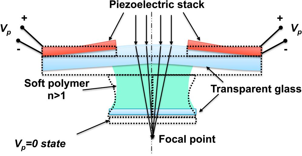

Figure 2 shows a planar view of symmetric actuator configurations for tunable lenses with different pupil geometries. Each of them is mounted on a clamped square diaphragm with a side length $a = 3 mm$ . A geometrical parameter $γ$ for each pupil’s actuator is defined as the ratio $L_{r} / a$ , where $L_{r}$ is the reference dimension marked by red arrows in Fig. 2. Specifically, in case 6, $L_{r}$ equals its circular opening diameter $2 c$ . For all study cases, the light passes only through the pupil opening area.

Fig. 2

Planar view of possible study cases of piezoelectrically actuated tunable lenses. A clamped square diaphragm with: (a) square, (b) 45-deg rotated square, (c) hexagonal, (d) octagonal, (e) 22.5-deg rotated octagonal, and (f) circular pupils. The red arrows indicate the reference dimension $L_{r}$ for each pupil.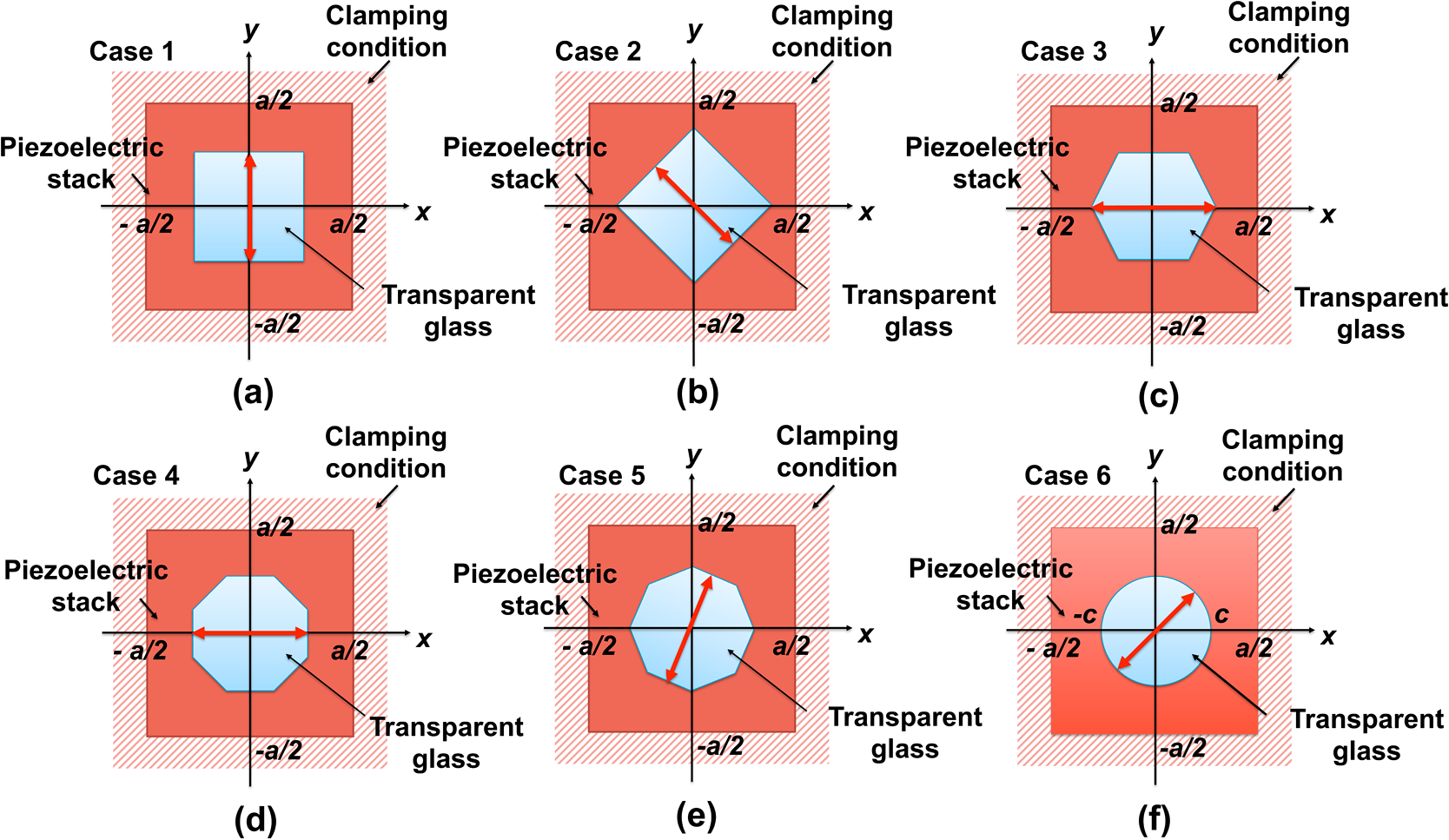

3. Electromechanical Modeling and Simulations

3.1.

Variational Formulation and its Solutions

In a previous research work,¹⁵ we have developed a variational formulation based on the classical laminated plate theory, linear piezoelectricity, quasielectrostatic conditions, and a thin film approximation. Originally, it was used to predict the displacement profile of the transparent membrane in case 6 [refer to Fig. 2(f)] taking into account the complicated geometry of its piezoelectric actuator. However, this variational formulation can be amended to predict the deformation caused by piezoelectric actuators with arbitrary openings. Here, we limit our concern to the polygonal-shaped openings, as in cases 1 to 5 shown in Fig. 2.

The variational method involves a minimization of an energy functional to find an approximate solution to the membrane displacement in the $z$ -direction $w_{0}$ . This displacement is approximated by a variational solution $w_{N}$ that is written as a linear combination of $N^{2}$ basis functions $ϕ_{m n} (X, Y)$ , such as

Eq. (1)

w_{0} (X, Y, 0) \approx w_{N} (X, Y, 0) = \sum_{m = 0}^{N - 1} \sum_{n = 0}^{N - 1} C_{m n} ϕ_{m n} (X, Y),

where

C_{m n}

are coefficients to be determined. Weighted Gegenbauer polynomials were chosen as basis functions in order to satisfy the clamped boundary conditions of zero deflection and zero slope along the diaphragm edges.¹⁵ In addition, they are orthogonal and easily mapped to Zernike polynomials, which suits an optical representation of wavefronts. For case 6, with all

γ

values of interest, we have previously found that

N = 28

is sufficient to obtain less than

10 %

l_{2}

relative error norm when comparing the displacement from the variational solution against FEM.¹⁵ This observation still holds for the other polygonal-shaped pupils.

Due to the mirror symmetries of the lens, we will only consider the even Gegenbauer polynomials, i.e., only functions where both indices $m$ and $n$ are even. The first four even polynomials can be expressed as follows:

Eq. (2)

ϕ_{00} = {(1 - X^{2})}^{2} {(1 - Y^{2})}^{2},

Eq. (3)

ϕ_{20} = \frac{9}{2} (11 X^{2} - 1) {(1 - X^{2})}^{2} {(1 - Y^{2})}^{2},

Eq. (4)

ϕ_{02} = \frac{9}{2} (11 Y^{2} - 1) {(1 - X^{2})}^{2} {(1 - Y^{2})}^{2},

Eq. (5)

ϕ_{22} = \frac{81}{4} (11 Y^{2} - 1) (11 X^{2} - 1) {(1 - X^{2})}^{2} {(1 - Y^{2})}^{2} .

Using weighted Gegenbauer basis functions to minimize the energy functional amounts to solving the linear system of equations:

Eq. (6)

[R_{m n p q}] [C_{m n}] = [F_{p q}],

where

[R_{m n p q}]

and

[F_{p q}]

are, respectively, the linear stiffness matrix and the effective force matrix and can be expressed as integrals (see Ref. 15 for further details). The flexural rigidity varies over the diaphragm due to the difference in layer structures between the actuator and the pupil areas. We follow the same modeling procedure as before except that the flexural rigidity expressions [Eq. (9) in Ref. 15] are put in a more general form:

Eq. (7)

D_{i j}^{*} = D_{i j}^{gl} + D_{i j}^{p} \bar{ζ} (X, Y),

where

D_{i j}^{gl}

is the flexural rigidity for the glass layer only, and

D_{i j}^{p}

is for the piezoelectric layer including the piezoelectric coupling within the piezoelectric material.

X = x / (a / 2)

and

Y = y / (a / 2)

are the normalized Cartesian coordinates. The complementary pupil function

\bar{ζ} (X, Y)

is 0 over the opening and 1 elsewhere. From Eq. (7), the quantities

D_{i j}^{*}

vary over the plate due to the difference in layer structure between the lens pupil and the actuator areas. The function

\overline{ζ}

serves as an integration mask in Eq. (7) allowing numerical calculations of the variational integrals to treat various pupil geometries on the same footing.

3.2.

Variational Solutions versus Finite Element Method Simulations

In the analyzed study cases, we have used the same material and structure dimensions for the square diaphgram and the piezoelectric actuator stack as in Ref. 15. We have considered a {100}-textured ${PbZr}_{0.53} {Ti}_{0.47} O_{3}$ thin film¹⁷ as the piezoelectric material and glass as the transparent layer. The PZT layer is $2 μ m$ thick and has a 100-nm bottom electrode from Pt {100} grown on 10-nm thick ${Ti / TiO}_{2}$ adhesion layers. Platinum electrodes and adhesion layers are neglected in calculations due to their small thicknesses compared to both glass and PZT layers.

For electromechanical simulations, the $γ$ values are varied from 0.1 to 0.9 for all pupils except for the square openings whose values were varied from 0.1 to 0.7. Beyond $γ = 1 / \sqrt{2}$ , the case-2 square pupil will cross the diaphragm boundaries. Figure 3 shows how the variational solutions (with $N = 28$ ) for all cases match with FEM simulations. Thus, they qualitatively provide good prediction for deflection to be used subsequently in optical simulations. The presented modeling framework provides a fast tool, compared to FEM, to perform optimization and exploration of different materials, layer thicknesses, and pupil geometries. For example, on our computer (Intel i7-4940MX, 3.1 GHz, 64-bit OS), the software package MATLAB¹⁸ solves Eq. (6) in 1.3 s while it takes 1.5 min to solve the corresponding problem with FEM (using COMSOL Multiphysics v4.4¹⁹).

Fig. 3

Displacement profiles in $x z$ -plane from FEM simulations and the variational solutions ( $N = 28$ ) for a clamped square diaphragm with (a) square, (b) 45-deg rotated square, (c) hexagonal, (d) octagonal, (e) 22.5-deg rotated octagonal, and (f) circular pupils at different $γ$ ratios with $V_{p} = - 10 V$ .

4. Optical Performance using Ray Tracing Analysis

We perform ray tracing analysis using Zemax,²⁰ an optical simulation tool. Both the glass and polymer (or fluid) layers have a refractive index equal to 1.5 and are assumed to have a unit optical amplitude transmittance within the visible light range. In the ray-tracing analysis, parallel rays uniformly illuminate the tunable lens’ entrance pupil opening, which is set as a stop surface limiting the ray bundle entering the lens. For polygonal-shaped pupils, a “user defined aperture”²⁰ was used to limit light rays to the polygonal-shaped pupil area only. In Zemax, the simulated ray bundle diameter was set equal to the polygon’s circumscribed circle diameter $γ_{op} a$ , where $γ_{op}$ is the ratio of the simulated optical ray bundle diameter to the diaphragm side $a$ . Based on the physical pupil geometry, it is defined as

Eq. (8)

γ_{op} = {\begin{cases} \frac{L_{p}}{a \sin (π / p)} & Polygonal - shaped pupil \\ γ = \frac{2 c}{a} & Circular pupil \end{cases},

where

L_{p}

is the polygon side length,

p

is the number of polygonal sides, and

2 c

is the diameter of the circular pupil. In the following, whenever we use the term “focal length,” we mean the distance from the lens’ flat face to the minimum on-axis spot. We do not use the paraxial approximation to calculate the focal length.

4.1.

Design Criterion: Minimum $F #$

A quantitative figure of merit for tunable lenses is the minimum achievable $F #$ with acceptable RMSWFE. For all the study cases, we calculate $F$ -number using an effective equation:

Eq. (9)

F # = \frac{f}{\sqrt{\frac{4}{π} A}},

where

f

is the focal length and

A

is the pupil area. Figure 4(a) shows the arrangement used in Zemax to determine the focal length and RMSWFE for the tunable lens. We imported a

512 \times 512

point grid of the lens’ surface sag from variational solutions and FEM simulations for comparison. Using the modeling framework, we search for the geometrical parameter

γ

that minimizes the

F

-number. For a fair comparison, we compare different lenses at the same pupil area to capture the same amount of light. The area of each polygon is

A_{f} \times a^{2}

, where

A_{f}

is an area factor defined as follows:

Eq. (10)

A_{f} = {\begin{cases} γ^{2} & Cases 1 and 2 \\ 3 \sqrt{3} γ^{2} / 8 & Case 3 \\ 2 γ^{2} / (1 + \sqrt{2}) & Cases 4 and 5 \\ π γ^{2} / 4 & Case 6 \end{cases} .

Fig. 4

(a) Tunable lens arrangement for on-axis optical simulations. (b) Reciprocal $F #$ and (c) RMSWFE versus the area factor $A_{f}$ for different pupils using variational solutions and FEM simulations, all with $V_{p} = - 10 V$ and $λ = 550 nm$ .

Figures 4(b) and 4(c) show deviations between optical performance from variational solutions and FEM simulations due to the relatively small errors in profiles shown in Fig. 3. $F #$ simulations show small deviations, but RMSWFE simulations suffer from larger deviations due to having the error in displacements comparable to the wavelength. Nevertheless, the optical parameters from variational solutions show the same trends as the FEM results. In addition, optimum values of the variational solutions $γ_{v}^{*}$ are very near to the optimum values of FEM simulations $γ_{FEM}^{*}$ , as shown in Table 1. The circular pupil ( $γ_{FEM}^{*} = 0.57$ ) achieves the minimum $F #$ of 129 among all cases with an RMSWFE of 0.0137 waves. In addition, it has the largest aperture area, which allows a wider ray bundle to be captured by the lens.

Table 1

Optimum γv* and γFEM* corresponding to minimum F# for variational solutions and FEM simulations, respectively. The Af, F#, and RMSWFE correspond to γFEM* values for tunable lens with polygonal and circular pupils at Vp=−10 V.

Pupil	γv*	γFEM*	Af	F#	RMSWFE (waves)
1	0.51	0.5	0.25	143.96	0.1183
2	0.5	0.49	0.24	146.93	0.1009
3	0.64	0.61	0.24	134.51	0.0505
4	0.57	0.55	0.25	129.43	0.0155
5	0.58	0.55	0.25	129.35	0.0168
6	0.59	0.57	0.26	129.04	0.0137

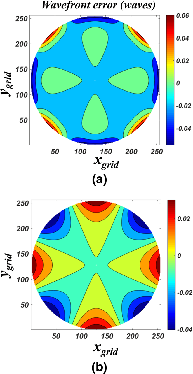
Table 2 lists the first six dominant aberrations and their percentage ratio $k_{m n}^{2} / \sum_{i, j} k_{i j}^{2}$ for each actuator case, where $k_{m n}$ is a coefficient of Zernike polynomial $Z_{n}^{m}$ evaluated at the exit pupil. For $γ_{FEM}^{*}$ values, as shown in Fig. 5, the on-axis wavefront error map differs based on the pupil geometries. The error maps display the combined symmetries of the square-diaphragm with the differently shaped pupils. It is evident that case 6 is dominated, with weight 99%, by the Zernike-quadrafoil aberration $Z_{4}^{4}$ that results from clamping conditions at the four edges. A point of interest for the circular pupil case is that a single Zernike aberration can be easily corrected to minimize the RMSWFE,²¹ when compared to other pupils.

Table 2

First six dominant aberrations at the exit pupil and their percentage for study cases with optimum value γFEM*.

	γ	1		2		3		4		5		6
Case 1	0.5	$Z_{4}^{2}$	14.79	$Z_{2}^{2}$	14.75	$Z_{4}^{4}$	12.35	$Z_{6}^{6}$	10.23	$Z_{6}^{2}$	9.52	$Z_{2}^{0}$	5.43
Case 2	0.49	$Z_{0}^{0}$	32.26	$Z_{4}^{4}$	28.03	$Z_{2}^{0}$	22.43	$Z_{4}^{0}$	5.1	$Z_{6}^{4}$	3.75	$Z_{6}^{0}$	2.78
Case 3	0.61	$Z_{0}^{0}$	67.2	$Z_{2}^{0}$	17.27	$Z_{4}^{4}$	3.84	$Z_{6}^{6}$	3.89	$Z_{12}^{12}$	2.8	$Z_{4}^{0}$	1.18
Case 4	0.55	$Z_{4}^{4}$	42.64	$Z_{8}^{8}$	31.61	$Z_{0}^{0}$	18.11	$Z_{2}^{0}$	6.81	$Z_{6}^{4}$	0.3	$Z_{16}^{16}$	0.21
Case 5	0.55	$Z_{4}^{4}$	45.84	$Z_{8}^{8}$	31.73	$Z_{0}^{0}$	15.89	$Z_{2}^{0}$	5.87	$Z_{6}^{4}$	0.25	$Z_{16}^{16}$	0.24
Case 6	0.57	$Z_{4}^{4}$	99.18	$Z_{6}^{4}$	0.5	$Z_{0}^{0}$	0.23	$Z_{2}^{0}$	0.06	$Z_{2}^{2}$	0.01	$Z_{8}^{8}$	$8.8 \times 10^{- 4}$
Pupil-masked case 2	$γ = 0.7$ , $γ_{op} = 0.7$	$Z_{4}^{4}$	45.14	$Z_{6}^{4}$	43.65	$Z_{8}^{8}$	5.49	$Z_{0}^{0}$	4.23	$Z_{2}^{0}$	1.4	$Z_{10}^{8}$	0.04
Case 6	0.7	$Z_{4}^{4}$	97.8	$Z_{6}^{4}$	1.41	$Z_{0}^{0}$	0.53	$Z_{2}^{0}$	0.17	$Z_{8}^{8}$	$4 \times 10^{- 3}$	$Z_{2}^{2}$	$9.14 \times 10^{- 4}$

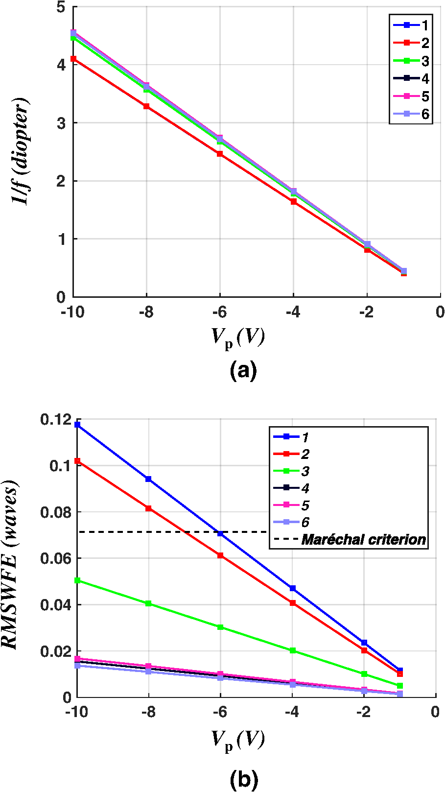
Fig. 5

Wavefront error map using exit pupil shape for (a) square, (b) 45-deg rotated square, (c) hexagonal, (d) octagonal, (e) 22.5-deg rotated octagonal, and (f) circular pupils with optimum $γ_{FEM}^{*}$ values at 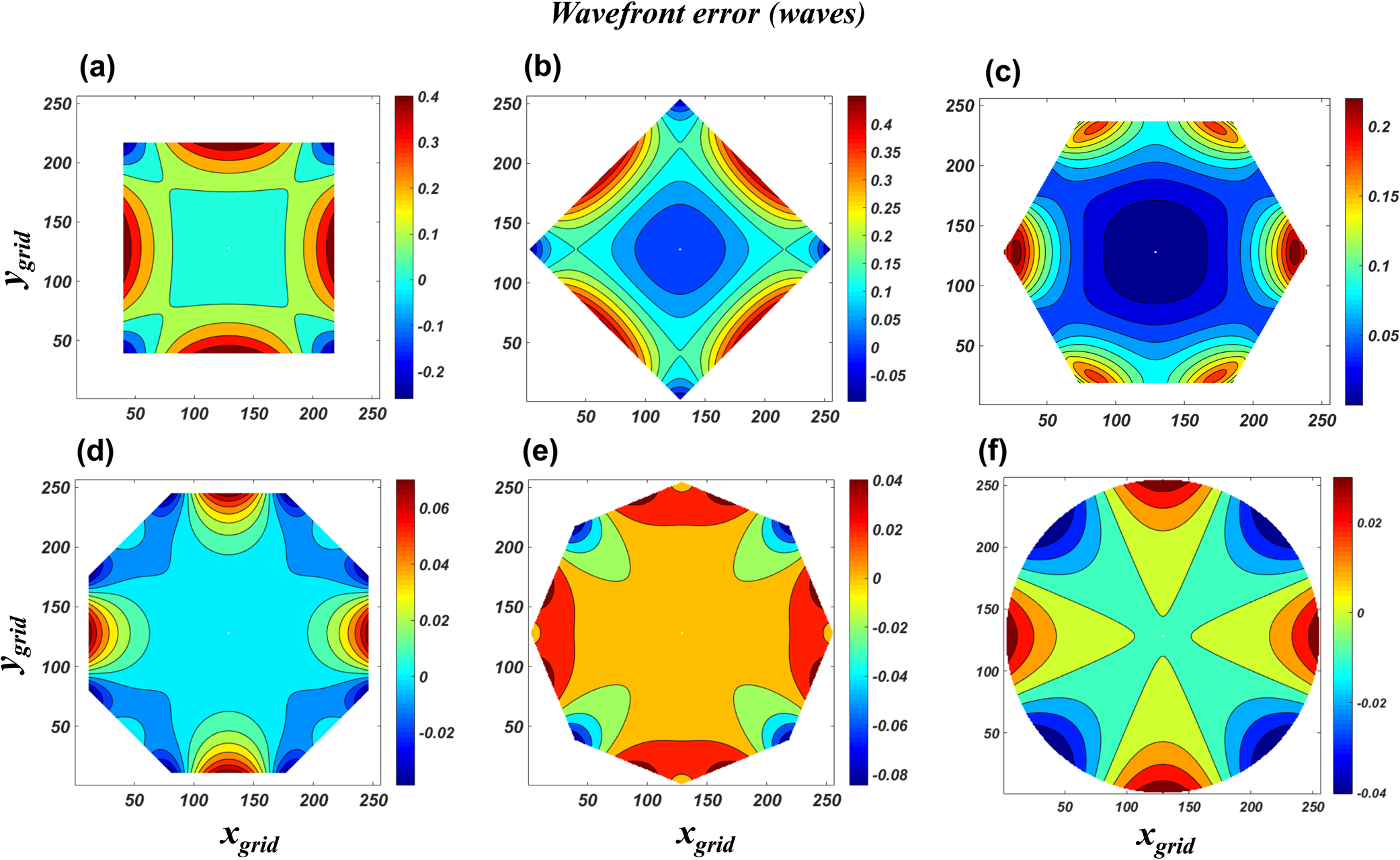$V_{p} = - 10 V$ .

Figure 6(a) shows that the achievable diopteric power is nearly 4.5 diopter with optimum geometrical parameters as the voltage is varied from 0 to $- 10 V$ . The voltage was limited to $- 10 V$ to comply with the assumptions that the deflection is mainly due to bending and that nonlinear coupling is insignificant. All cases suffer from a wavefront error whose RMS value depends linearly on the voltage, as shown in Fig. 6(b). This linear dependency is due to having the displacement profiles, by assumption, linearly dependent on voltage. The introduced RMSWFEs in cases 3 to 6 are very small compared to the threshold value $λ / 14$ defined by Maréchal’s criterion to judge whether the performance is diffraction-limited or not.²²

Fig. 6

(a) Lens dioptric power $1 / f$ and (b) RMSWFE versus the applied voltage on the piezoelectric stack with optimum $γ$ values for all tunable lens cases.

4.2.

Tunable Lens Combined with a Fixed Lens

To study the tunable lens at the system level, such as for smartphone camera application, we combine it with a fixed lens, as shown in Fig. 7(a). Their combination enable us to put an object at different focus positions from the camera, refocus by adjusting the actuation voltage on the tunable lens, and calculate the overall MTF at the image plane. Over the focusing range, it is desirable that the overall MTF does not become worse than the MTF of the fixed lens alone. The resolution of the captured image would be consequentially independent of the object distance. For an initial design, we picked a fixed lens¹⁶ that was designed with constraints on $F #$ and for aberration corrections in portable imaging devices. It had a focal length of 3.55 mm, $F$ -number of 2.2 and FOV of $\pm 78 \deg$ . We have modified the original design to have a focal length equal to 4 mm and an opening diameter of 2 mm. The maximum FOV was kept unchanged. The details of the modified design are summarized in Table 3. For these optical simulations, we have chosen the circularly shaped tunable lens that achieves the minimum $F #$ among all cases. It has an opening diameter of 1.71 mm and achieves 22.1 cm focal length at $- 10 V$ . However, their combination gives the best focus at a distance 36.8 cm instead due to the fixed lens’ own aberrations and its influence on the minimum spot size distance.

Fig. 7

(a) Arrangement of the tunable lens with a fixed lens in Zemax for optical simulations. Sagittal and (tangential) MTF for (b) the fixed lens alone without movement when the object is located at infinity and 368 mm at different field points on the image plane (coordinates are given in mm in legends). MTF for the tunable lens with circular pupil and the fixed lens when the object is located away (c) 1103 mm, (d) 552 mm, and (e) 368 mm.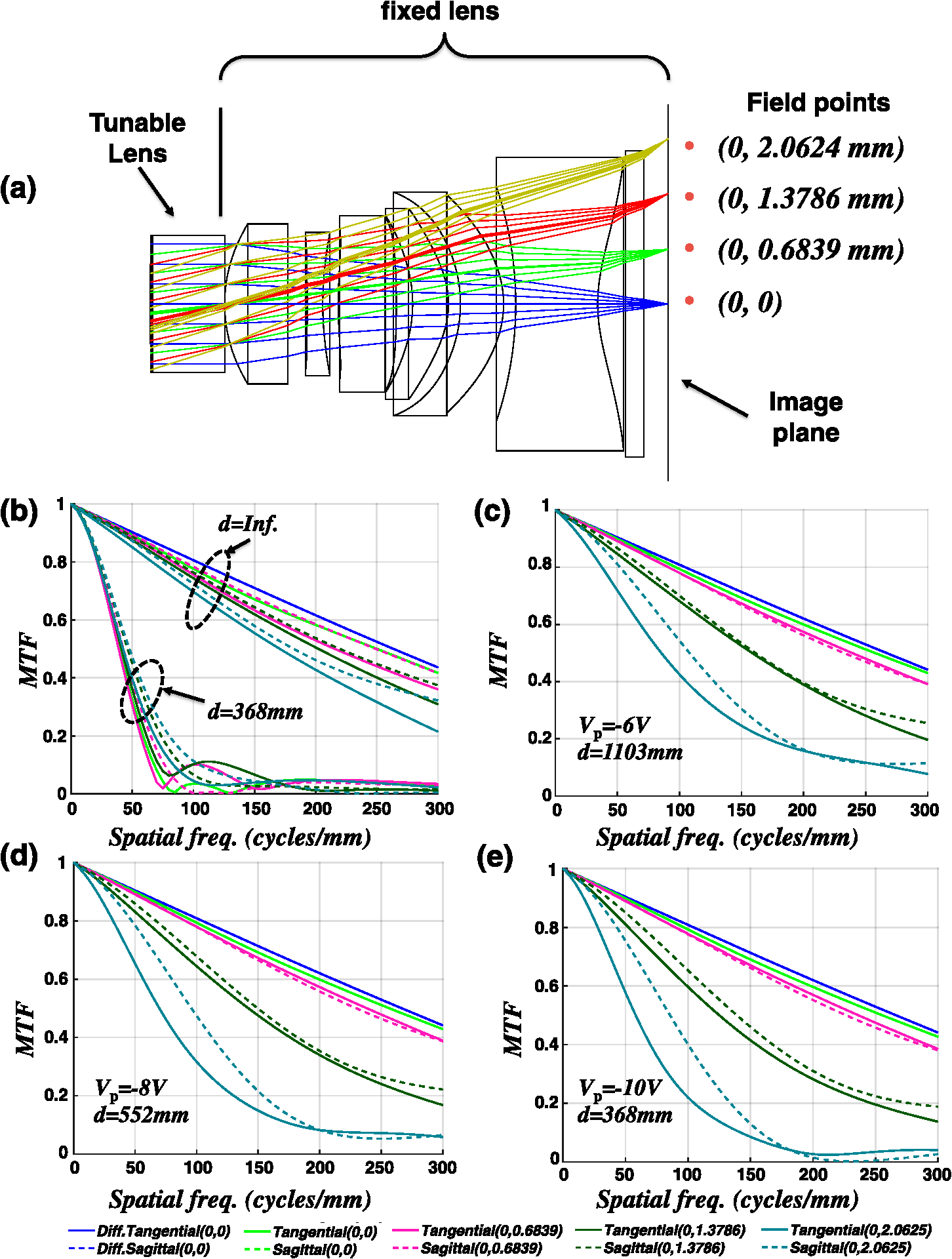

Table 3

Details of the modified fixed lens (dimensions are in mm).

Surface	Radius	Thickness	(nd,νd)	Semidiameter	Conic constant	4th order	6th order	8th order	10th order	12th order
1a	1.856	0.782	(1.53, 56)	1	0.135	$- 7463 \times 10^{- 3}$	0.014	$- 0.022$	0.014	$- 8.596 \times 10^{- 3}$
2	27.592	0.242		0.82	−624.814	$3.773 \times 10^{- 3}$	$- 0.028$	$- 7.137 \times 10^{- 3}$	$- 0.011$	$4.481 \times 10^{- 3}$
3	$- 138.585$	0.194	(1.63, 23)	0.852	$1.547 \times 10^{4}$	$- 0.017$	$- 9.477 \times 10^{- 3}$	$- 0.014$	$- 0.028$	0.025
4	4.031	0.192		0.894	$- 23.018$	0.013	$3.336 \times 10^{- 3}$	$- 4.356 \times 10^{- 3}$	$- 0.01$	0.014
5	5.22	0.722	(1.53, 56)	0.941	$- 46.639$	$- 0.038$	$- 0.019$	$- 2.323 \times 10^{- 3}$	$- 5.511 \times 10^{- 3}$	$2.537 \times 10^{- 3}$
6	$- 11.777$	0.203		1.102	$- 222.236$	$- 0.032$	$- 0.027$	$2.195 \times 10^{- 3}$	$- 3.87 \times 10^{- 3}$	$- 1.822 \times 10^{- 3}$
7	$- 1.646$	0.444	(1.53, 56)	1.104	$- 2.167$	0.01	$4.525 \times 10^{- 4}$	$- 6.106 \times 10^{- 3}$	$8.394 \times 10^{- 5}$	$- 3.163 \times 10^{- 3}$
8	$- 1.08$	0.149		1.194	$- 2.427$	$8.527 \times 10^{- 3}$	$- 3.672 \times 10^{- 3}$	$4.695 \times 10^{- 3}$	$- 1.567 \times 10^{- 3}$	$- 1.71 \times 10^{- 3}$
9	$- 1.663$	0.536	(1.63, 23)	1.4	$- 2.541$	$- 0.023$	$- 0.026$	$9.408 \times 10^{- 5}$	$5.217 \times 10^{- 3}$	$- 3.87 \times 10^{- 3}$
10	$- 1.289$	0.151		1.363	$- 1.364$	$- 2.731 \times 10^{- 3}$	$- 6.671 \times 10^{- 3}$	$- 3.915 \times 10^{- 4}$	$3.196 \times 10^{- 4}$	$9.747 \times 10^{- 5}$
11	$- 4.461$	1.018	(1.63, 23)	1.464	2.828	$5.432 \times 10^{- 3}$	$2.824 \times 10^{- 3}$	$- 1.815 \times 10^{- 3}$	$4.151 \times 10^{- 4}$	$- 2.902 \times 10^{- 5}$
12	1.924	0.344		1.835	$- 6.748$	$- 0.034$	0.01	$- 1.865 \times 10^{- 3}$	$1.542 \times 10^{- 4}$	$- 5.173 \times 10^{- 6}$
13	Inf	0.228	(1.52, 64.2)	1.846	—	—	—	—	—	—
14	Inf	0.326		1.913	—	—	—	—	—	—
IMA	Inf			2.063	—	—	—	—	—	—

^aFixed lens’ aperture stop surface.

Figure 7(b) shows the MTF of the fixed lens alone both when the object is at infinity and when it is 368 mm away. The MTF has dropped significantly for the closer object because of the larger defocus term $Z_{2}^{0}$ in the wavefront error. Combining the fixed lens with the circularly shaped tunable lens will preserve the MTF performance from significant degradation over a range of object distances after refocusing, as shown in Figs. 7(c) to 7(e). The tunable lens keeps the MTF nearly the same at different object positions. However, a closer look at the combined MTF shows that the performance is diffraction limited up to the field point (0, 0.6839 mm) that corresponds to a $\pm 10 - \deg$ FOV. Beyond that angle, the MTF drops due to the tunable lens’ off-axis aberrations. For a larger FOV, a simultaneous redesign of the tunable and fixed lens would be helpful to compensate for the dominant aberration.

4.3.

Lens Dioptric Power and RMSWFE Tradeoff: Pupil Masking

Pupil masking can affect a lens’ figure of merits, such as RMSWFE, dioptric lens power $1 / f$ , pupil area, resolution, and contrast. Thus, it can be used as a design degree of freedom to make tradeoffs. Therefore, we have explored masking the polygonal-shaped pupils by a circular mask. This can be done during device fabrication by having the PZT stack’s lower Pt electrode as a circular opening instead of having the same polygonal shape as the rest of the PZT actuator layers, such as in cases 1 to 6. Figure 8 shows a pupil-masked case 2 as an example. Light will only pass through the circular opening in the lower Pt electrode layer. The pupil-masked case 2 is now geometrically parametrized by two parameters: $γ$ for the piezoelectric actuator and $γ_{op}$ for the circular opening in the lower Pt electrode. $γ$ still equals $L_{r} / a$ . However, $γ_{op}$ in this pupil-masked case 2 will follow the circular pupil definition from Eq. (8), which equals $2 c / a$ (refer to Fig. 8).

Fig. 8

(a) Planar view of pupil-masked case 2. (b) Cross-sectional view showing the 45-deg rotated square actuator with its circular lower Pt electrode etched to form a circular pupil. The red arrow indicates the reference dimension $L_{r}$ for each pupil. The blue arrow indicates the diameter $2 c$ for the circular pupil opening in the lower Pt electrode.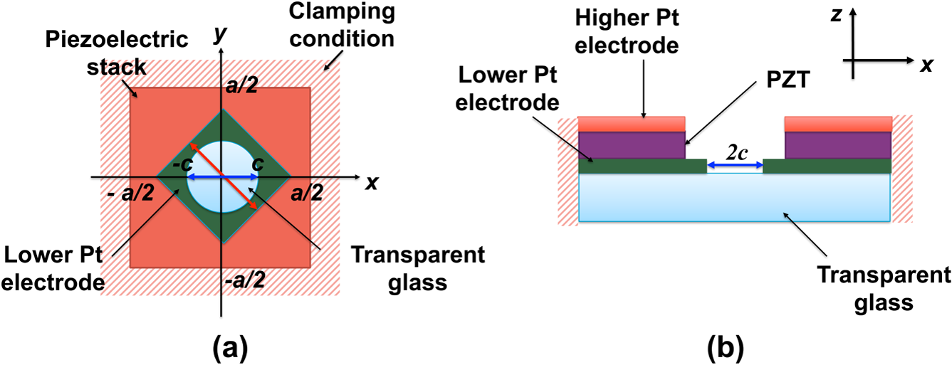

We have neglected the effect of platinum and adhesion layers on the lens displacement. Thus, for optical simulations, we just do a parametric sweep on $γ_{op}$ for each $γ$ value. The $γ_{op}$ values are kept below $L_{p} / [a \tan (π / p)]$ , which corresponds to the polygon’s inscribed circle. As a result of this parametric sweep, we get the scattering plots for RMSWFE and $1 / f$ in Figs. 9(a) and 9(b).

Fig. 9

Scattering plots of (a) RMSWFE and (b) lens dioptric power $1 / f$ with varying the ratios 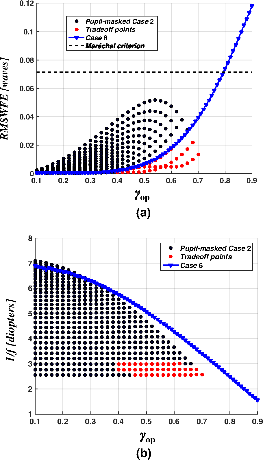$γ_{op}$ and $γ$ , all with $V_{p} = - 10 V$ and $λ = 550 nm$ .

We have picked case 6 as a reference since it achieves the minimum $F #$ , as previously discussed. We compare pupil-masked case 2 versus case 6 with the same pupil opening diameter in Figs. 9(a) and 9(b). It is evident that pupil-masked case 2, compared to case 6, provides a tradeoff between dioptric power and RMSWFE, specifically for large apertures marked as red dots. They offer lower RMSWFE but less dioptric power for large apertures when compared to case 6. An example on tradeoff points is case 2 with $γ = γ_{op} = 0.7$ that achieves $f = 389 mm$ and RMSWFE of 0.0133 waves. A comparable case 6 with $γ = 0.7$ has the same pupil diameter, achieves $f = 293 mm$ and $RMSWFE = 0.0395$ waves, which is a 1 diopter better $1 / f$ but 3.4 times worse RMSWFE. Their wavefront error map is shown in Fig. 10 and their dominant aberrations are listed in Table 2.

Fig. 10

Wavefront error map for (a) pupil-masked case 2 with $γ = 0.7$ and $γ_{op} = 0.7$ . (b) Case 6 with $γ = 0.7$ .

Exploring pupil masking for the other cases (1 and 3 to 6) shows no benefits compared to case 6 without pupil masking. All the explored cases give higher RMSWFE and lower dioptric power than the reference case.

5. Conclusion

The modeling framework has been effectively used after an amendment to predict the linear static optoelectromechanical performance of complicated actuator configurations for piezoelectrically actuated tunable lenses. Thus, it can be utilized for the optimization of different material choices, layers thicknesses, and pupil geometries to find the optimum geometrical ratio $γ$ that achieves the minimum $F$ -number with acceptable RMS wavefront error.

Among different pupil geometries, the tunable lens with circular pupil has the widest aperture area with an area factor 0.26 compared to the square diaphragm area. It achieves nearly 4.5 diopters with a 10-V voltage source and has an RMS wavefront error less than the Maréchal’s criterion. Its aberrations are 99% dominated by quadrafoil Zernike aberration that can be easily balanced. Its MTF response combined with a fixed lens remains unaffected for a $\pm 10 - \deg$ FOV when the object is located at different distances after actuation voltage adjustment. Beyond the $\pm 10 - \deg$ , the MTF response is degraded due to off-axis aberrations.

Pupil masking, for the actuator with a $45- \deg$ rotated square opening, achieves tradeoffs between lens dioptric power and RMSWFE for larger apertures when compared to the actuator with circular opening without pupil masking.

Acknowledgments

The authors thank the Research Council of Norway and PoLight AS for financial support. The Research Council of Norway (Grant no. 235210).

References

1.

Y. Tseng, “Voice coil motor apparatus,” U.S. Patent No. 7,400,068 (2008).

2.

C. Zhao, Ultrasonic Motors: Technologies and Applications, Science Press and Springer-Verlag, Berlin Heidelberg (2011). Google Scholar

3.

M. Ye, B. Wang and S. Sato, “Liquid-crystal lens with a focal length that is variable in a wide range,” Appl. Opt., 43 6407 –6412 (2004). http://dx.doi.org/10.1364/AO.43.006407 APOPAI 0003-6935 Google Scholar

4.

N. Chronis et al., “Tunable liquid-filled microlens array integrated with microfluidic network,” Opt. Express, 11 2370 –2378 (2003). http://dx.doi.org/10.1364/OE.11.002370 OPEXFF 1094-4087 Google Scholar

5.

A. Werber and H. Zappe, “Tunable microfluidic microlenses,” Appl. Opt., 44 3238 –3245 (2005). http://dx.doi.org/10.1364/AO.44.003238 APOPAI 0003-6935 Google Scholar

6.

S. Kuiper, “Variable-focus liquid lens for portable applications,” Proc. SPIE, 5523 100 (2004). http://dx.doi.org/10.1117/12.555980 PSISDG 0277-786X Google Scholar

7.

U. Wallrabe, “Axicons et al.—highly aspherical adaptive optical elements for the life sciences,” in 2015 18th Int. Conf. on Solid-State Sensors, Actuators and Microsystems (TRANSDUCERS 2015), 251 –256 (2015). http://dx.doi.org/10.1109/TRANSDUCERS.2015.7180909 Google Scholar

8.

K. Haugholt et al., “Polymer lens,” U.S. Patent No. 8,199,410 (2012).

9.

J. Wohlstadter, “Method of and apparatus for generating a 3-D image from a 2-D image having a changeable focusing micro-lens array,” U.S. Patent No. 5,986,811 (1999).

10.

J.-Y. Son and B. Javidi, “Three-dimensional imaging methods based on multiview images,” J. Disp. Technol., 1 125 (2005). Google Scholar

11.

T. Furukawa, Biological Imaging and Sensing, Springer, Heidelberg, Germany (2004). Google Scholar

12.

E. T. Koufogiannis, N. P. Sgouros and M. S. Sangriotis, “Perspective rectification of integral images produced using arrays of circular lenses,” Appl. Opt., 52 4959 –4968 (2013). http://dx.doi.org/10.1364/AO.52.004959 APOPAI 0003-6935 Google Scholar

13.

J. Kim et al., “Liquid crystal-based square lens array with tunable focal length,” Opt. Express, 22 3316 –3324 (2014). http://dx.doi.org/10.1364/OE.22.003316 OPEXFF 1094-4087 Google Scholar

14.

N. Chen et al., “Resolution comparison between integral-imaging-based hologram synthesis methods using rectangular and hexagonal lens arrays,” Opt. Express, 19 26917 –26927 (2011). http://dx.doi.org/10.1364/OE.19.026917 OPEXFF 1094-4087 Google Scholar

15.

M. A. Farghaly, M. N. Akram and E. Halvorsen, “Modeling framework for piezoelectrically actuated MEMS tunable lenses,” Opt. Express, 24 28889 –28904 (2016). http://dx.doi.org/10.1364/OE.24.028889 OPEXFF 1094-4087 Google Scholar

16.

S. Lai and C. Lee, “Six-piece optical lens system,” (2013). Google Scholar

17.

N. Ledermann et al., “1 0 0-textured, piezoelectric $Pb ({Zr}_{x} {Ti}_{1 - x}) O_{3}$ thin films for MEMS: integration, deposition and properties,” Sens. Actuators A, 105 (2), 162 –170 (2003). http://dx.doi.org/10.1016/S0924-4247(03)00090-6 Google Scholar

18.

MathWorks, (2017) https://www.mathworks.com/products/matlab.html February ). 2017). Google Scholar

19.

COMSOL Multiphysics, Stockholm, Sweden (2013). https://www.comsol.com Google Scholar

20.

Washington, USA (2015). Google Scholar

21.

G. Dai, Wavefront Optics for Vision Correction, SPIE Press, Bellingham, Washington (2008). Google Scholar

22.

A. Maréchal, “Etude des influences conjuguées des aberrations et de la diffraction sur l’image d’un point,” (1947). Google Scholar

Biography

Mahmoud A. Farghaly is currently a PhD researcher at the University College of Southeast Norway. He received his BA and MSc degrees in electrical engineering from Assiut University, Egypt, in 2010 and 2013, respectively. His current research interests include design and modeling of MEMS sensors and actuators for mobile phones, such as (Lorentz-force and inductive) magnetometers and piezoelectric actuators.

Muhammad Nadeem Akram is a professor at the University College of Southeast Norway. He obtained his PhD in photonics from Royal Institute of Technology, Stockholm, Sweden, in 2005. His research interests are semiconductor lasers, imaging optics, laser projectors, and speckle reduction.

Einar Halvorsen is a professor of micro- and nanotechnology at the University College of Southeast Norway. He received his Siv. Ing. degree in physical electronics from the Norwegian Institute of Technology (NTH) in 1991 and his Dr. Ing. degree in physics from the Norwegian University of Science and Technology (NTNU, formerly NTH) in 1996. Since then, he has worked both in academia and the microelectronics industry. His current research interests are in theory, design, and modelling of microelectromechanical devices.

CC BY: © The Authors. Published by SPIE under a Creative Commons Attribution 4.0 Unported License. Distribution or reproduction of this work in whole or in part requires full attribution of the original publication, including its DOI.

Citation Download Citation

Mahmoud A. Farghaly, Muhammad Nadeem Akram, and Einar Halvorsen "Optical performance of piezoelectrically actuated MEMS tunable lenses with various pupil geometries," Optical Engineering 56(3), 035104 (21 March 2017). https://doi.org/10.1117/1.OE.56.3.035104

Received: 15 December 2016; Accepted: 28 February 2017; Published: 21 March 2017

Access the abstract

JOURNAL ARTICLE
10 PAGES

DOWNLOAD PAPER SAVE TO MY LIBRARY

GET CITATION

CITATIONS

Cited by 7 scholarly publications.

Explore citations on Lens.org

KEYWORDS

Microelectromechanical systems

Lenses

Finite element methods

Modulation transfer functions

Actuators

Wavefronts

Refractor telescopes

1.

Introduction

2.

Principle of Operation

Fig. 1

Fig. 2

3.

Electromechanical Modeling and Simulations

3.1.

Variational Formulation and its Solutions

Eq. (1)

Eq. (2)

Eq. (3)

Eq. (4)

Eq. (5)

Eq. (6)

Eq. (7)

3.2.

Variational Solutions versus Finite Element Method Simulations

Fig. 3

4.

Optical Performance using Ray Tracing Analysis

Eq. (8)

4.1.

Design Criterion: Minimum F#

Eq. (9)

Eq. (10)

Fig. 4

Table 1

Table 2

Fig. 5

Fig. 6

4.2.

Tunable Lens Combined with a Fixed Lens

Fig. 7

Table 3

4.3.

Lens Dioptric Power and RMSWFE Tradeoff: Pupil Masking

Fig. 8

Fig. 9

Fig. 10

5.

Conclusion

Acknowledgments

References

Biography

Show All Keywords

Keywords/Phrases

Search In:

Publication Years

Design Criterion: Minimum $F #$