|
|
1.IntroductionIn recent years, there has been a particular interest in research on dazzling by continuous-wave laser radiation. It is highly probable that this interest is correlated to the increasing proliferation of handheld high-power laser pointers. For example, Williamson1 put a lot of effort into the investigation of the influence of laser dazzle on the human eye. Besides work on computer visualization of laser eye dazzle and the study of the influence of atmospheric scattering on human eye dazzle,2 they introduced the very interesting concept of the “nominal ocular dazzle distance.”3 This approach allows the calculation of the minimum distance for the detection of targets in case of laser dazzle. Coelho et al.4 developed a computer model of the eye to assess laser dazzle. Besides investigations regarding laser dazzle of the human eye, laser dazzle of electro-optical sensors is quite interesting since they are highly susceptible to laser illumination. The realization of protection measures encountering laser irradiation of arbitrary wavelength is not an easy task. Conventional laser protection measures like absorbing or interference filters usually work only for specific wavelengths or a limited spectral range. Therefore, for wavelength-independent laser protection measures, other techniques have to be utilized. An overview on different possibilities for laser protection is given in a publication of Svensson et al.5 A very important issue is the maximum attenuation of laser radiation that can be achieved with a protection measure. However, in the case of imaging systems, the characterization of laser protection measures solely by assessing such a simple number is by far not sufficient. Usually, (effective) protection measures always introduce some disturbances (e.g., color distortions) that can lead to poor image quality. Such drawbacks will not be considered by these measurements, but a severe loss of image quality can highly reduce the sensor’s performance. Thus, it is also necessary to examine how much information can be retained from a dazzled image of a hardened sensor for an adequate evaluation of the protection measure. Considering that, a new method is necessary to determine the loss of information in dazzled sensor images. Different applications are imaginable for such a method, yet in general, two (slightly) different issues shall be addressed:
In this publication, we examine three different data analysis methods to quantify the amount of laser dazzling in sensor images (see Sec. 2). In order to analyze their applicability to the evaluation of laser protection measures, dazzling experiments (see Sec. 4) were performed with two different sensors at four laser wavelengths (488, 515, 561, and 640 nm). Both sensors entail an optical setup making them less vulnerable to laser dazzling (see Sec. 3). 2.Methods to Quantify Laser Dazzling2.1.Overexposed Pixel CountingSchleijpen et al.6–8 used an easy applicable method to quantify sensor dazzling. They estimated an equivalent diameter of the overexposed part in dazzled images as a function of laser irradiance and camera integration time. This diameter is derived by counting the number of overexposed pixels in the sensor image and subsequently calculating the diameter of a disc containing the same number of pixels. 2.2.Pattern RecognitionDurécu et al.9,10 used an approach for their quantitative assessment of laser dazzled CCD cameras, where cameras observed a scene containing a number of different characters (“N,” “H,” “E,” “U,” “V”). These characters had to be recognized by a pattern recognition algorithm. The algorithm was based on either correlation9 or Fourier descriptors.10 Hueber et al.11 also used pattern recognition algorithms to quantify laser dazzling of thermal imagers. For our work, we adapted this approach to our needs. Instead of a test chart consisting of characters, we decided to utilize test charts consisting of triangular optotypes according to the “triangle orientation discrimination” (TOD) method.12 TOD is a common method to characterize the performance of electro-optical systems. Triangular optotypes oriented in four possible orientations (up, down, left, or right) are presented to observers, which have to indicate the triangle orientation. The results of such observer tests, performed with triangles of different size and contrast, allow deriving specific sensor characteristics. In the case of imagers working in the visible spectrum, it represents the minimum resolvable contrast (MRC), whereas in the case of thermal imagers, it is the minimum resolvable temperature difference (MRTD). Although these characteristic sensor parameters (MRC and MRTD) are not within the scope of our work, we combined the triangular optotypes of the TOD method with the pattern recognition approach. We decided to analyze the sensor images rather by an automatic image analysis algorithm than by human observers to avoid time-consuming observer tests. Thus, the choice of a specific optotype is of less importance. However, the use of triangular optotypes still offers the possibility to present the same data to human observers for further analysis or for evaluation purposes, if needed. For the image analysis, we used a correlation-based template matching algorithm in order to recognize equilateral triangles of different sizes, which can be oriented in four different orientations as mentioned before. The task of the image analysis algorithm was to discriminate the orientation of triangles in dazzled sensor images. 2.3.Structural Similarity IndexAs a third method to quantify laser dazzling, we analyzed the image data by calculating the structural similarity (SSIM) index. The SSIM index is a metric for measuring the quality of an image by comparing it to a distortion-free reference image.13 This metric is based on the assumption that the human visual system is designed to recognize structures in images and to estimate to what extent two images exhibit the same structures. Usually, SSIM is used to assess the quality of image compression algorithms. In our case, images taken with a camera dazzled by laser light are compared to an image taken without laser dazzling. Thus, we get a measure of how much image information can be retrieved when applying a particular protection measure. 3.Tested SensorsTwo sensors were tested: a sensor hardened by the use of a digital micromirror device (DMD; see Sec. 3.1) and a sensor based on complementary bands (see Sec. 3.2). 3.1.Hardened Sensor Based on a Digital Micromirror DeviceThis sensor is hardened against laser dazzling by an optical setup, including a DMD14 and wavelength multiplexing.15 Detailed information about this sensor can be found in various publications.16–22 Here, only a short introduction to the hardened sensor shall be given. A scheme of the optical setup is shown in Figs. 1(a) and 1(b); a photograph of the hardened sensor is shown in Fig. 1(c). The heart of the sensor is a DMD, which allows intensity modulation. In order to be able to filter light only in localized areas of the sensor’s field-of-view, the DMD is located at the intermediate focal plane of a Keplerian telescope formed by lenses L1 and L2. Before and behind the telescope, two identical dispersive elements (gratings Gr1 and Gr2) are placed along the optical beam path to implement the wavelength multiplexing and demultiplexing. The first grating spectrally disperses the light beams entering the setup in such a way that each object point of a distant scene forms a wavelength spectrum at the intermediate focal plane of the telescope. Then, in order to reconstruct the image, the dispersion induced by the first grating has to be reversed behind the telescope what is realized by means of the second grating. Fig. 1Concept for hardening a sensor against laser dazzling using a DMD: (a) operation mode for regular imaging, (b) operation mode with high attenuation of dazzling laser light, and (c) photograph of the hardened sensor. 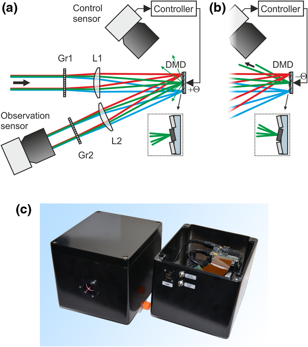 Without dazzling laser light, this setup is operated in such a way that all light entering the lens is directed toward the sensor by having all micromirrors tilted to the -state [Fig. 1(a)]. In the case when dazzling laser light arrives at the sensor (here: the green rays in the figure), the controller toggles solely those micromirror elements to the -state that are exposed with dazzling light [Fig. 1(b)]. Thus, the dazzling light is reflected out of the regular beam path, whereas all remaining wavelengths, originating from the same object point as the dazzling laser radiation, can still pass unaffected through the optical arrangement. Light originating from other object points remains unaffected on all wavelengths as far as these wavelengths are not directed to those micromirrors toggled to the -state. Thus, the method of wavelength multiplexing allows combined spatial and spectral filtering of monochromatic light. The mean attenuation in the spectral range between 470 and 725 nm was measured to be 45.5 dB.17 In the case of laser dazzle, the controller automatically activates the micromirrors in order to filter out the unwanted laser radiation. The automatic activation is achieved by monitoring stray light generated at the DMD when illuminated by monochromatic laser radiation. As monitor, a dedicated control sensor17 (monochrome CMOS camera) is utilized. Using this technique, the knowledge of exact laser wavelength and the position of the laser source within the field of view is not required. The filtering of laser radiation is illustrated in Fig. 2 by four images taken with the hardened sensor. In the images, a test chart can be seen without [Fig. 2(a)] and with laser dazzle [Figs. 2(b)–2(d)] and, in the case of dazzling, with different numbers of activated micromirrors. Although the switching rate of the DMD is specified as 22,727 Hz when using in 1-bit-mode, the reaction time of the controller is limited by the (adjustable) integration time of the control sensor. The integration time is usually in the order of some tens of milliseconds. Fig. 2Images taken with the hardened sensor (a) without and (b–d) with laser dazzle (laser wavelength , radiant exposure ). The numbers of activated micromirror elements are indicated. 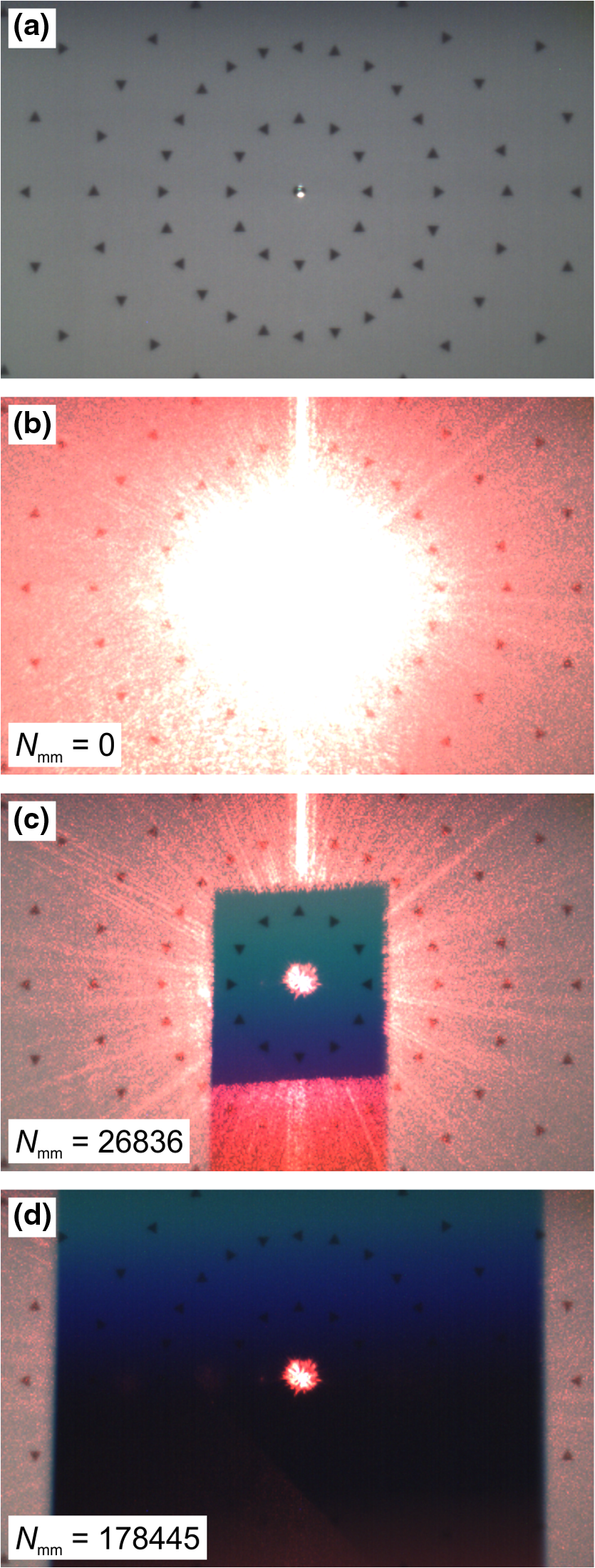 The micromirrors necessary to attenuate laser dazzling are always activated according to the scene. Although the DMD is driven automatically by the controller, there is still one free parameter in the algorithm, which is chosen by the user: the number of activated micromirrors to cover the laser spot on the DMD. According to the value of this parameter, a smaller or larger part within the sensor’s field of view is filtered. This has a significant influence on the resulting image. If is large, the filtered area covers a large field-of-view. However, there is a reasonable loss of contrast and brightness in the sensor image [see Fig. 2(d)]. If only a small number of micromirrors is activated (low value of ), the filtered area is limited to a small field of view [see Fig. 2(c)], but the contrast in the filtered part is much higher compared to the case before. This issue will come up again in Sec. 5 and in the discussion of the measurement results in Sec. 6.1. 3.2.Sensor Based on Complementary BandsThe second sensor we evaluated makes use of complementary bands.5 Incoming light is divided into a number of spectrally separated bands, and for each spectral band, a dedicated imaging sensor is used. If the spectral separation of the bands was chosen appropriately (monochromatic), dazzle laser light will only jam the corresponding spectral channel. An algorithm detects the dazzling and suppresses the overexposed pixels. Thus, in the superimposed image (all channels are fused), the overexposed pixels are not taken into account and the result is a dazzle-free image. Such an approach does not really represent a “protection measure” in the classical way since a dazzle laser is still able to jam one of the sensors. However, the output of the system still allows an observer to fulfill his task without a strong loss in image quality. A laboratory demonstrator based on this approach was built with three spectral bands (three-band-sensor). A sketch of the optical layout is shown in Fig. 3(a). The incoming light first passes a Keplerian telescope formed by the camera lens (Schneider-Kreuznach Apo-Xenoplan 2.0/35-2001, , ) and the internal lens L1 (). Subsequently, the light is spectrally split into three different optical channels by the use of two dichroic beam splitters (DBS500 and DBS600). Each channel represents a different spectral band: blue channel ( to 500 nm), green channel ( to 600 nm), and red channel ( to 700 nm). Besides the spectral separation by these dichroic beam splitters, an additional use of shortpass (SPxxx) and longpass filters (LPxxx) in each optical channel ensures that outband laser radiation is effectively attenuated. Finally, the light in each channel is focused by lenses L2 () on the imaging sensors (VRmagic VRmMS-12 using an Aptina MT9V024 CMOS imaging sensor). Fig. 3(a) Schematic diagram of the optical layout of the three-band-sensor. (b) and (c) Photographs of the three-band-sensor (without external camera lens).  Please note, in contrast to the schematic diagram of Fig. 3(a) representing the functional principle of the sensor system, the shortpass filter SP700 may be placed in front of lens L1, acting than as an IR cut-off filter for the whole system. Photographs of the laboratory demonstrator (built up with standard optomechanical components) can be seen in Figs. 3(b) and 3(c). The external camera lens is not present in these images. The sensor system is powered and controlled via USB connection by an external computer. The computer retrieves the three separate sensor images and computes a fused image. The image fusion algorithm is principally based on a simple calculation of mean pixel values from the three single images. However, prior to the calculation of the mean values, the algorithm examines if in a single spectral band saturation of pixels occurs due to narrowband light radiation. In the case that monochromatic dazzle occurs, only the not-saturated pixels are taken into account for the calculation of the mean value. This is depicted in Fig. 4. Fig. 4Images taken by the three-band-sensor: (a) blue, (b) green, (c) red channel (laser wavelength , radiant exposure ), and (d) final image resulting out of the fusion of the three channels. 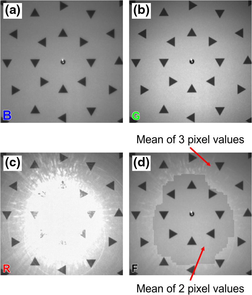 Figures 4(a)–4(c) show the color channel images taken by the three-band-sensor (B: blue channel, G: green channel, R: red channel). The sensor system was illuminated with laser radiation (wavelength ; radiant exposure ) resulting in a dazzle spot in the red channel. For the fused image in Fig. 4(d), the overexposed pixels of the red channel were not taken into account for the calculation of the mean value. Thus, in the center part of the fused image, the mean value was calculated just by the two pixel values of the blue and green channel. Still, the triangles in the center part of the fused image are clearly visible. For an observer, the occurrence of laser dazzle is perceptible by the darker center as only two pixel values comprise the mean value. This darker region is the result of differences in the responsivity of the different channels. The signal of a particular channel depends on the corresponding optics transmittance and the integration time of the sensor. Since the optical elements in the three channels are different, differences of the transmittance are compensated by adjusting the integration time. For the measurements, the integration times were set to 6.5, 9.0, and 8.0 ms for the red, green, and blue channels, correspondingly. At best, there would be the same signal when the sensor system looks at a homogenous background. However, the setting of the imaging sensor’s integration times could not be accomplished perfectly, especially due to different vignetting in the three channels. Calculated values for transmittance and optical density of the three optical channels are shown in the graphs of Fig. 5. These data were computed from the transmittance curves of the optical elements as specified by the manufacturer. Fig. 5Calculated optical properties of the three-band-sensor: (a) transmittance and (b) optical density as a function of wavelength. The laser wavelengths used for the laboratory measurements are marked by orange colored, vertical lines. The passbands of the three channels are highlighted by colored background. 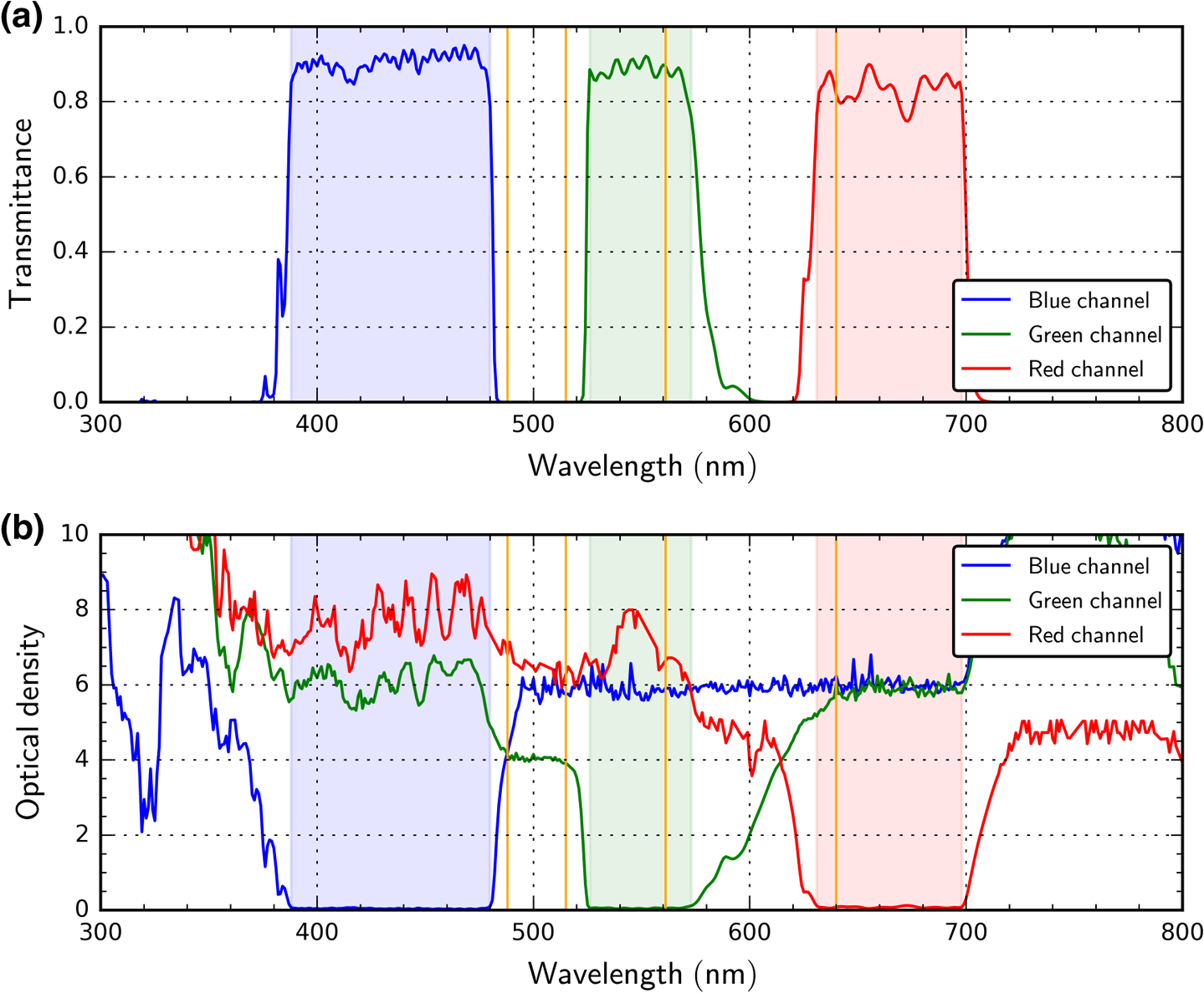 In order to get spectrally well-separated channels, the edges of the shortpass and longpass filters must be very steep and cannot be chosen to be exactly 500 or 600 nm. Otherwise, the optical density at the crossover point of the filter curves would not be high enough to attenuate laser radiation effectively at these wavelengths. Therefore, the filters were picked in such a way that outband laser radiation is attenuated by six orders of magnitude. The passbands of the three channels (defined as transmittance ) are marked by colored background. The laser wavelengths used in the experiments (488, 515, 561, and 640 nm, see Sec. 4) are marked in the graphs by orange colored, vertical lines. Two of the available laser wavelengths (488 and 515 nm) are spectrally located in the stopband between the passbands of the blue and green channel. Thus, for the three-band-sensor only, the two longer wavelengths could be used for dazzling measurements. 3.3.Sensor ParametersA comparison of the parameters of both the hardened sensor and the three-band-sensor is given in Table 1. Table 1Parameters of the two sensors used in the experiments.
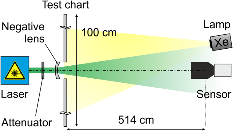
4.Experimental Setup4.1.Laboratory MeasurementsMost of our laser dazzling evaluation experiments were performed in the laboratory using dedicated test charts. A sketch of the experimental setup is shown in Fig. 6. The sensor under the test observed the test charts (size ) from a distance of 514 cm. The test charts were only partly seen by the sensor due to the limited sensor’s field-of-view (see Table 1). A hole of 15 mm diameter in the center of the test charts allowed illuminating the sensor with laser radiation along the sensor’s optical axis. For the dazzling, we used a multiwavelength laser source iChrome MLE-L from Toptica. This device comprises four different lasers (wavelengths 488, 515, 561, and 640 nm) with output powers ranging from 40 mW up to 100 mW. Each of the laser outputs is coupled into a common single-mode fiber. The fiber’s output was collimated using an off-axis parabolic mirror (Thorlabs RC12APC-P01) to avoid chromatic aberration. Subsequently, a lens with a negative focal length (, Thorlabs LF1547-A or , Thorlabs LF1544-A) spread the laser beam to overspill the sensor’s optics. The laser power was set to the desired values by means of two filter wheels equipped with neutral density filters offering a maximum optical density of 5.3. The test chart was illuminated with the light of a xenon arc lamp (Asahi Spectra MAX-303). The illuminance at the center of the test chart (measured on the optical axis) was about 400 lx. As test charts, we used white boards of diffuse scattering characteristics with an imprinted pattern consisting of equilateral triangles. Five different test charts were prepared, each showing triangles of a different size. Figure 7 shows a sketch of one of the test charts. The diameters of the circumscribed circles of the different triangle sizes were chosen to correspond to angles of 0.5, 0.4, 0.3, 0.2, and 0.1 deg as seen from the sensor’s position. In TOD, the stimulus size of a triangle is usually defined as the square-root area of the triangle. This value can be calculated from the diameter of the circumcircle (in units of mrad) by , resulting in stimulus sizes of 5.0, 4.0, 3.0, 2.0, and 1.0 mrad. The geometrical arrangement of the triangles was designed to be located on concentric circles around the optical axis (see Fig. 7). Seen from the sensor’s position, the radii of the concentric circles increase in steps of 1 deg. Fig. 7Sketch of a test chart used for the laboratory experiments (triangle size 0.4 deg). Triangles of one size with different orientation are aligned on five concentric circles with eccentricities ranging from 1 to 5 deg. For each triangle size (diameter of the circumscribed circle ranging from 0.1 to 0.5 deg), a separate test chart was prepared. 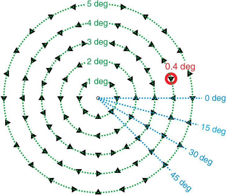 In our previous work, we used just a single test chart offering triangles of three different sizes and two different contrasts.23 It became apparent that this choice of test chart was not optimal for the data analysis since for each combination of eccentricity, triangle size and contrast only four triangles were available on the test chart. Thus, when calculating the fraction of correct orientation discrimination, the resulting values corresponded to the limited set {0, 0.25, 0.5, 0.75 1.0}, but not to other values. We also recognized that the two different contrast values chosen for the “old” test chart had only little influence on the results. Therefore, for the current analysis, we limited the contrast of the triangles to one value and prepared separate test charts for the different sizes of triangles. The measurement procedure was always as follows:
In case of the hardened sensor under dazzling, images were taken with and without activation of the DMD. This allows an evaluation of the performance of this protection concept. Additionally, for each value of radiant exposure, the number of activated micromirrors was changed in order to achieve optimal protection. The term “optimal protection” is to be understood in the sense of the highest recognition rate that can be attained in dependence of the number of activated micromirrors. 4.2.Field TrialA further outcome of our earlier work made us realize that a test chart with homogeneous background and a sparse number of triangles does not fit to a SSIM analysis (see Sec. 5.3). The reason is that such a test chart represents a scene with quite low amount of structures in it, whereas the SSIM index measures the similarity of structures. A richly structured scene is more suitable for this kind of data analysis. Therefore, we also used data from an earlier field trial showing a real scene17 for the SSIM method. Figure 8 shows some images taken from a video sequence captured with the hardened sensor (see Sec. 4.1). The scene consists of a container on a meadow in front of a metal fence [see Fig. 8(a)]. Some cars are parked along a road in the background. Fig. 8Images taken at a field trial with the hardened sensor: (a) scene without disturbing laser radiation, (b) scene with laser dazzle; the protection measure (DMD) was not activated, (c) scene with laser dazzle; the protection measure (DMD) was activated. 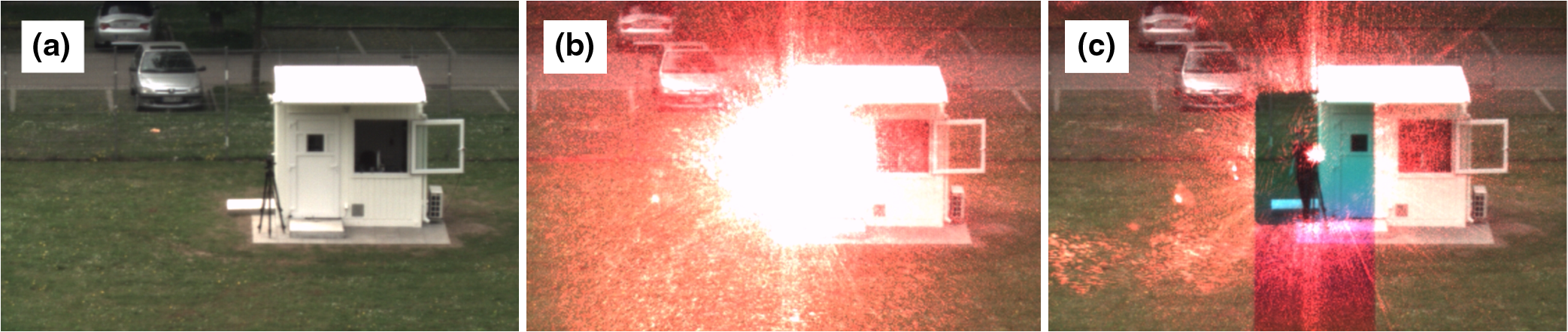 A continuous wave laser (wavelength: 660 nm, output power: 2.7 mW, divergence: ) was placed in front of the container at a distance of 73 m to the sensor. When the laser was switched on, a large part of the central field of view was completely dazzled [see Fig. 8(b)]. As soon as the control loop of the system was activated, the dazzling laser radiation was strongly attenuated [see Fig. 8(c)]. Because of the operating principle, a band of wavelengths is suppressed in the imaging path, resulting in a color distortion, but scene details in close vicinity to the laser (e.g., the person operating the laser) are visible. 5.Data AnalysisThe analysis of the image data was performed according to the three different methods, as already mentioned in Sec. 1: (1) overexposed pixel counting (OPC, see Sec. 5.1), TOD (see Sec. 5.2), and calculation of the SSIM index (see Sec. 2.3). The results of the image analysis are processed slightly different for the two sensors:
5.1.Overexposed Pixel CountingUsually, the laser dazzle pattern in a sensor image is not rotationally symmetrical [see, e.g., Fig. 8(b)]. In order to state the size of the dazzled area, the number of overexposed pixels in sensor images is estimated and subsequently, the diameter of a disc containing the same number of pixels is calculated: The angular obscuration diameter (in radians) can then be calculated using the pixel pitch of the image sensor and the focal length of the camera lens: Since the size of the triangles is not important for this kind of analysis, the results of the measurement series for different triangle sizes were averaged. For the hardened sensor, only the best results (lowest obscuration radius) obtained by varying the number of activated micromirrors are plotted in the graphs of Sec. 6.1. 5.2.Triangle Orientation DiscriminationThe discrimination of the triangle orientation in the sensor images was accomplished by template matching based on cross-correlation calculations. The necessary templates for each size of triangle (0.1 to 0.5 deg) were extracted from undazzled images of the test charts. Then, regarding the different orientations of the triangles, the extracted templates were rotated by 90, 180, and 270 deg in order to get templates for all four possible orientations. The template matching was performed by computing successively the fast cross-correlation for each orientation of the triangles. By setting a suitable threshold , the cross-correlation algorithm estimated positions for the triangles of different orientation. Occasionally, it was possible for the algorithm to assign multiple orientations to a specific triangle on the test chart (i.e., the correlation values for two or more orientations were above the threshold ). In this case, we chose the orientation with the highest correlation coefficient as the result. It was also possible that a triangle was recognized at a position where no triangle existed. Such results were dismissed. The analysis procedure is visualized in Fig. 9. Fig. 9Image analysis by means of TOD: (a) an undazzled image is used to extract a template (orientation: up), (b) all other orientations (left, down, right) are generated by rotating the extracted template, (c) template matching is performed on an undazzled image to produce (d) a map of the triangle existing in the scene. (e) Example of template matching that is performed on a dazzled image.  In detail, the performed steps in our image analysis were as follows, explained by the example of the hardened sensor (, triangle size: 0.4 deg):
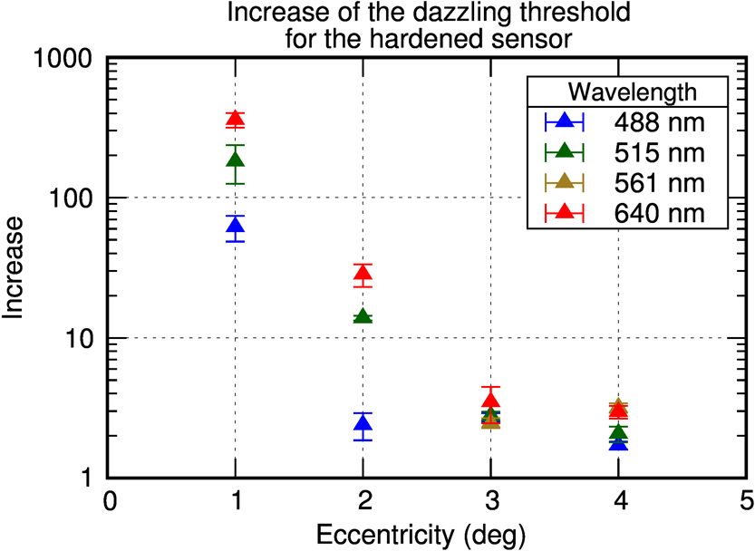
Fig. 10Fraction correct as a function of radiant exposure for the hardened sensor (triangle size: 0.4 deg, laser wavelength: 515 nm). The blue data points are the results with deactivated DMD (protection off); the red data points correspond to an activated DMD (protection on). Multiple red data points for a specific radiant exposure are due to different numbers of activated micromirrors . Error functions are fitted to the data points; for the protected case, the maximum values marked with circles are used for the fit. The values of radiant exposure where fraction correct reaches 75% are marked by vertical lines. 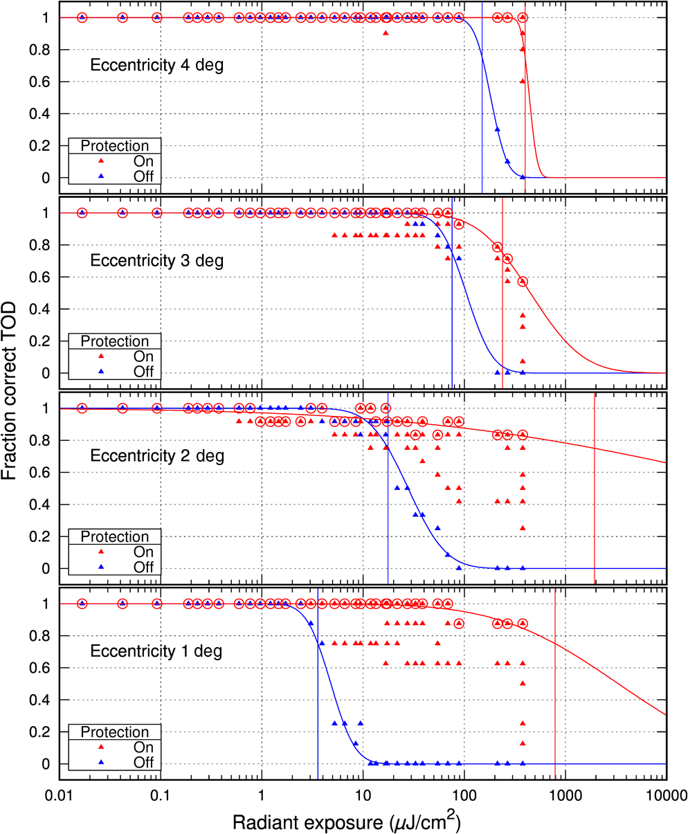 5.3.Structural Similarity IndexThe SSIM index is a method for measuring the similarity between two images and , and is computed according to the following equation:13 where is the average of , is the average of , is the variance of , is the variance of , is the covariance of and , and , . is the dynamic range of the pixel values (2bits per pixel-1) and , .Usually, Eq. (3) is applied to a small window of of the two images and , which is slid over the images to be evaluated. The result is the mean of the values computed for all single windows. In our case, the window length was . As for the OPC method, the results of the measurement series for different triangle sizes were averaged. For the hardened sensor, again only the best results (highest value of SSIM index) obtained by varying the number of activated micromirrors are plotted in the graphs of Sec. 6.1. 6.Results6.1.Results for the Hardened Sensor Based on a Digital Micromirror Device6.1.1.Overexposed pixel counting resultsFigure 11 shows the results of data analysis according to the OPC method for the hardened sensor. In Fig. 11(a), the obscuration radius is plotted as a function of radiant exposure. The color of the data points corresponds to the laser wavelength, their appearance represents the state of the protection mode (filled triangles: protection off, open triangles: protection on). When the obscuration radius exceeds 3 deg, the value of the obscuration radius starts to saturate, because the dazzle spot exceeds the geometrical dimensions of the imaging sensor. As can be seen also from that graph, the obscuration diameter decreases when the protection is activated. The amount of the decrease is plotted in Fig. 11(b). Fig. 11Results of the OPC method for the hardened sensor: (a) obscuration radius (in degrees) according to the OPC method for the protected and unprotected case. (b) Relative decrease of the obscuration radius (in percent) when the protection measure (DMD) is activated referred to the unprotected case. 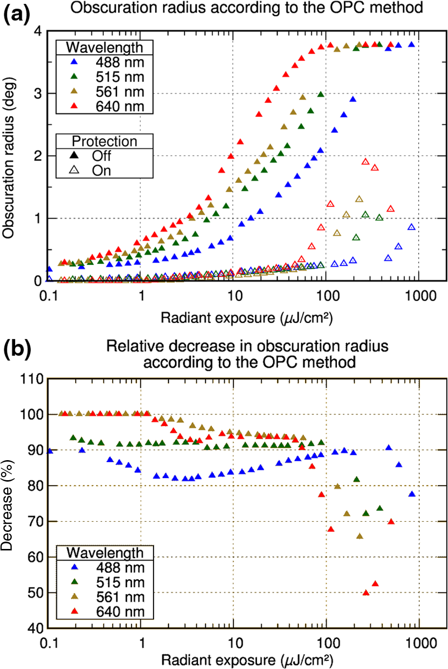 Figure 11(a) also reveals a shift of the curves depending on the laser wavelength. For longer laser wavelengths, the saturation of the sensor starts at lower values of radiant exposure. We will also see this behavior in the results of the other two methods (TOD and SSIM). This can be explained by the spectral characteristics of the hardened sensor. The radiant exposure needed to saturate a sensor pixel depends on the photon energy, the quantum efficiency of the imaging sensor, and the transmittance of the optical system, which are all wavelength-dependent. From the results of a theoretical calculation, we expect a ratio of the saturation thresholds of for the wavelengths 488, 561, 515, and 640 nm, which can qualitatively explain the shift of the curves. More details to the calculation can be found in the Appendix. 6.1.2.Triangle orientation discrimination resultsFigure 12 shows the obscuration radius as function of the radiant exposure for the hardened sensor, which is the result of the data analysis according to the TOD method. For each laser wavelength, a separate graph is presented. Filled and open data points correspond to the case of deactivated DMD (protection off) and activated DMD (protection on), respectively. The triangle size is represented by the size of the data points. Please note that no results are available for the triangle size of 0.1 deg since the template matching did not work reliably for this size of the triangles. This can be explained by the fact that the sensor’s optics is optimized at infinity and the optical components are not adjustable. In our experiments, the target’s distance was only 514 cm and thus, the test chart was not imaged perfectly on the DMD. Fig. 12Results of the TOD method for the hardened sensor: laser wavelength (a) 488 nm, (b) 515 nm, (c) 561 nm, and (d) 640 nm. 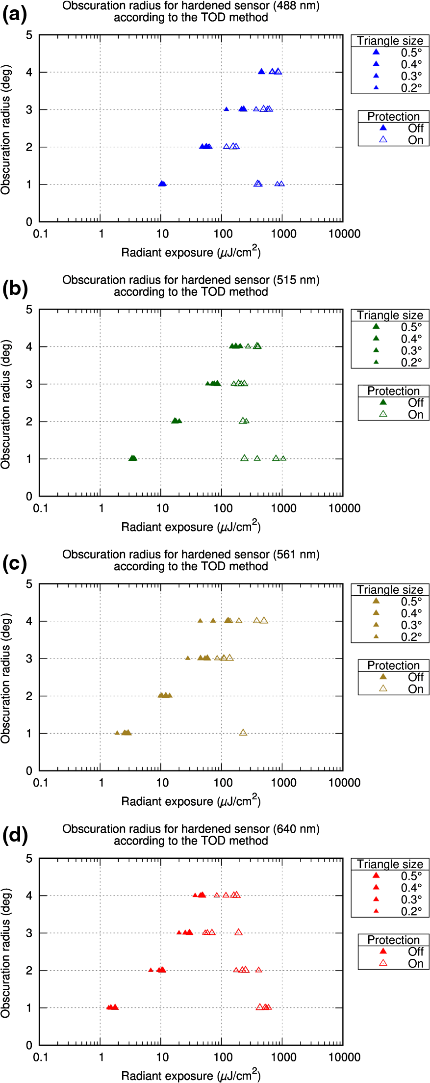 As can be seen from the graphs in Fig. 12, the size of the triangles has no significant influence on the results. This is true especially for the unprotected case (filled data points), where all data points for a specific obscuration radius lie at a very similar value of radiant exposure. For the protected case (open data points), we can see some differences. However, no particular trend can be observed, e.g., for large triangles, the dazzling occurs at higher values of radiant exposure than for small triangles. Just as for the OPC results, we can also discover a shift of the curves to lower values of radiant exposure for larger laser wavelengths. From the graphs, we can also see that the activation of the protection measure leads to an increased amount of radiant exposure necessary to dazzle a specific field of view of the sensor: the open data points are shifted to higher values of radiant exposure as compared to the filled data points. The smaller the dazzled area, the larger is the shift of the dazzling threshold. This behavior can be explained by the number of micromirrors that have to be activated to suppress the laser dazzle in different parts of the field of view. For example, in order to suppress the dazzle just to see the triangles on the 1 deg eccentricity-ring, only a small number of micromirrors have to be activated [see Fig. 2(c)]. This leads to a relatively high contrast and low color distortion in the filtered part of the field of view and finally results in a large shift of the dazzling threshold when the protection is activated. If a larger part of the field of view has to be filtered, e.g., to see the triangles on the 3 deg eccentricity-ring, a larger number of micromirrors have to be activated [see Fig. 2(d)]. This leads to low contrast and strong color distortion, preventing the perceptibility of the triangles. Thus, the shift of the dazzle threshold to higher values of radiant exposure is only small. But more importantly, the dazzle threshold is not reduced. Figure 13 shows the increase of the dazzling threshold for the hardened sensor. Since the triangle size has no extensive impact on the threshold values, they were averaged for this graph. 6.1.3.Structural similarity results of the laboratory measurementsThe SSIM results of the laboratory experiments for the hardened sensor are shown in Fig. 14. The graph in Fig. 14(a) shows the values of the SSIM index as a function of radiant exposure. Again, the colors of the data points correspond to the laser wavelength; the appearances of them represent the state of the protection mode (filled triangles: protection off, open triangles: protection on). The increase in the value of the SSIM metric when the protection is switched off compared to the unprotected case is shown by the graph in Fig. 14(b). Fig. 14Results of the SSIM analysis for the hardened sensor: (a) value of the SSIM index for the protected and unprotected case and (b) increase of the SSIM index (in percent) when the protection measure (DMD) is activated compared to the unprotected case. 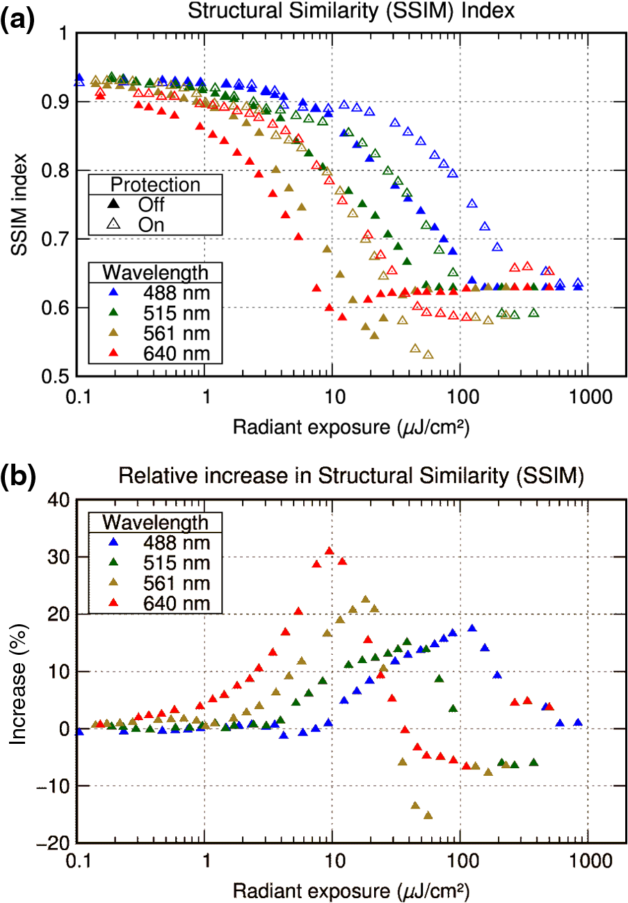 In Fig. 14(a), we can see that the SSIM index initially decreases with increasing radiant exposure. For higher values of radiant exposure, the SSIM index rises slightly and saturates to a fixed value. We attribute this behavior to the choice of our test chart. The test chart has a homogeneous, bright background with a sparse number of dark triangles on it. This means that the amount of structures is limited. When sensor dazzling starts, the disappearing triangles and the dazzle spot in the sensor image represent a change in structure, which is measured by the SSIM metric. However, for very large values of radiant exposure, the sensor image is (nearly) completely saturated. We then have the situation that the sensor image shows a homogeneous background (all pixels are white) again and just the sparse number of triangles is missing. Thus, the SSIM index is increased. 6.1.4.Structural similarity results for the field trial dataDuring a field trial, a video sequence was captured; three images of the sequence are shown in Fig. 8. For each image in the sequence, the SSIM index was calculated. The calculation was performed separately for each color channel and additionally, the mean of these three values was calculated. The graph in Fig. 15 shows the SSIM index versus the frame number for the different color channels and the mean value. The essential temporal events in time are marked by orange rectangles:
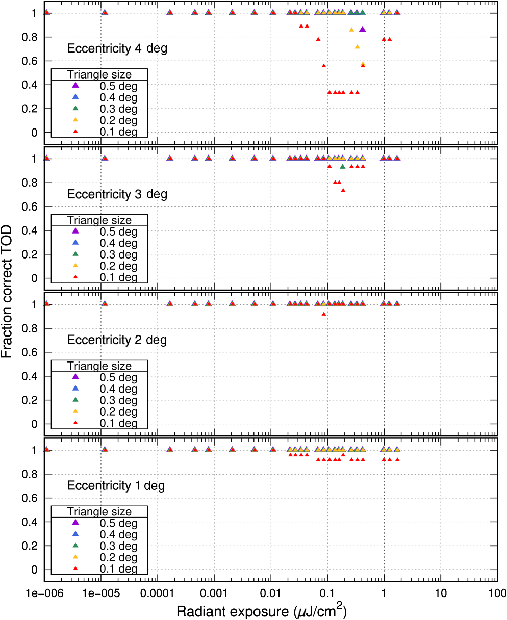
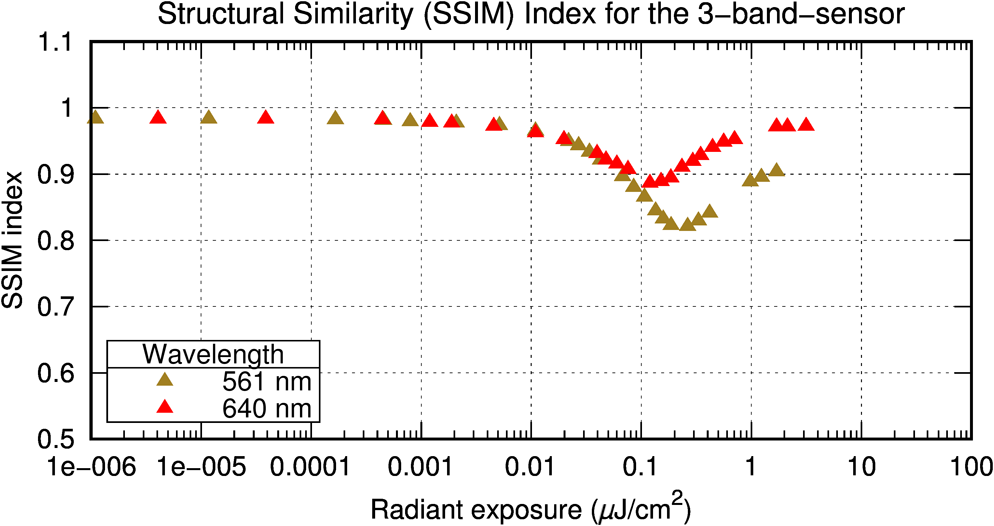
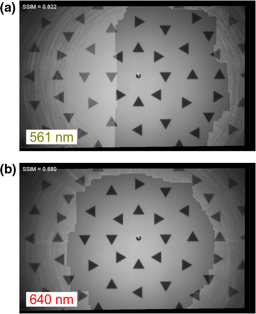
Fig. 15Results of the SSIM analysis for the hardened sensor. The SSIM index is plotted versus the frame number of a video sequence captured during a field trial. The four curves show the progress of the SSIM index for the three color channels (R: red, G: green, B: blue) and the mean of these three values (black curve). Specific events marked by orange rectangles: (1) laser is switched on; protection is deactivated; (2) protection is activated; (3) laser is switched off and protection is deactivated. 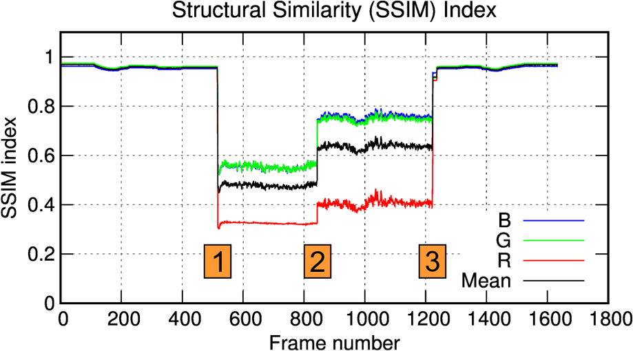 The increase in the SSIM index for the protected case (time frame 2–3) referred to the unprotected case (time frame 1–2) is 38% for the blue channel, 36% for the green channel, and 25% for the red channel. For the mean SSIM index, the increase is 33%. 6.2.Results for the Sensor Based on Complementary Bands6.2.1.Overexposed pixel counting resultsFor the three-band-sensor, no processible results according to the OPC method are available. Due to the operating principle of the fusion algorithm described in Sec. 3.2 (neglecting overexposed pixels for calculating the mean), no overexposed pixels exist in the output images that can be counted. For a single wavelength laser source, overexposure can only occur when the laser irradiance is that high that the out-of-band rejection of the complementary bands is not sufficient. In this case, also the imaging sensors of the complementary bands can be overexposed. Since the channel separation is in the order of 60 dB [see Fig. 5(b)], the laser irradiance has to be six orders of magnitude larger than the saturation irradiance for the in-band channel, which was not the case for the laser source used in the experiments. Therefore, no graphs can be presented here for that case. Overexposed pixels could also occur when using multiple laser sources with different laser wavelengths that fit to the passbands of the different channels. 6.2.2.Triangle orientation discrimination resultsThe results for the three-band-sensor, according to the TOD method, reveal a similar behavior of the three-band-sensor as for the OPC method. In Fig. 16, the fraction correct for laser illumination with wavelength is plotted as a function of radiant exposure. Only for the smallest triangles (size 0.1 deg), a noticeable effect can be seen, particularly for the eccentricity of 4 deg. In contrast to the hardened sensor, obscuration radii as a function of radiant exposure could not be extracted from these results. 6.2.3.Structural similarity resultsThe results of the SSIM analysis for the three-band-sensor (see Fig. 17) show a similar behavior as the OPC and TOD results. There is only weak influence of the laser irradiation on the value of SSIM; an effect is noticeable for a radiant exposure of roughly , where the SSIM index drops to minimum values of 0.82 and 0.88 for laser wavelengths of 561 and 640 nm, respectively. The corresponding images taken with the three-band-sensor are shown in Fig. 18. 7.Comparison of the Different ApproachesThe three methods used for data analysis are quite different, each one having its own advantages and disadvantages. The features of the three approaches are compared in Table 2. Table 2Comparison of the features of the different methods for data analysis.
The OPC method is very easy to implement and the effort necessary to realize the experimental setup is quite low. As a big advantage, no test chart is needed for this method. The method is based on the number of overexposed pixels as a function of radiant exposure. Using these numbers, the size (diameter or radius) of corresponding discs containing the same number of pixels is calculated. This disc is interpreted as the part of the field of view that is obscured by the laser dazzle spot generated on the detector. As we will see below, the results match quite well those of the more elaborate TOD method, presuming the sensor under test is not specifically protected. However, for the evaluation of a sophisticated protection measure like the one implemented by using a DMD in our hardened sensor, this method is limited. The pattern of active micromirrors can be highly inhomogeneous, resulting in a complex dazzle pattern on the sensor that cannot be described by a simple obscuration radius (or diameter). The TOD method allows a very detailed analysis of the information content in sensor images. This enables even the evaluation of such complex protection measures as mentioned before. However, the effort for the experimental setup and particularly for the data analysis is quite high. The advantage of the SSIM method lies in the evaluation of the information content in images of real scenes. No specific test chart is necessary, only care has to be taken that the sensor image exhibits enough structural information. The computation of the SSIM index is quite easy if programming libraries are available that already include a function for this task. The direct comparison of the results of the three methods is not easy since their output is quite different:
Both the TOD and the SSIM method evaluate the information content of sensor images. A comparison of the two results is not easy to derive because for the TOD method, the evaluation is conducted spatially resolved, whereas for the SSIM method, it is integrated. To compare the results, the TOD analysis could be integrated (computation of the fraction correct for the whole image instead separated for different eccentricities) or the SSIM method could be computed spatially resolved. For example, the SSIM index could be computed only for ring-shaped areas corresponding to the eccentricities [e.g., the areas within the white circles in Fig. 9(d)]. Since the TOD method allows the derivation of obscuration radii, these values can be compared with those of the OPC method. In Fig. 19, the comparison of results is shown for the hardened sensor (based on the use of a DMD) with deactivated protection. The lines in the plot correspond to the results regarding OPC data of Fig. 11(a). The data points show the TOD results. The filled triangles (oriented upwards) correspond to the result from Fig. 12, whereby the values for the different triangles sizes were averaged. Except for a laser wavelength of 640 nm, the data points do not match the lines. Fig. 19Comparison of obscuration radii derived with two different data analysis methods (OPC and TOD). In the case of the TOD method, two different levels of fraction correct (75% and 50%) were used to derive the values. 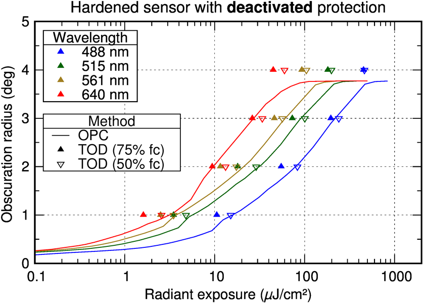 As explained in Sec. 5.2, the determination of the obscuration radius for the TOD method takes place by finding the value of radiant exposure, where the fraction correct equals 75%. If this analysis is performed by using only a required value of 50% for the fraction correct, we obtain slightly different obscuration radii. These radii are plotted in Fig. 19 as open triangles (oriented downward). Now, we receive a good correspondence of the data points with the lines for the laser wavelengths of 488, 515, and 561 nm. 8.SummaryIn order to assess laser dazzle of imaging devices, we compared three different approaches. In this context, two different home-built imaging sensors hardened against laser dazzling were investigated. The first approach (OPC) is based on the count of overexposed pixels in sensor images and the determination of an equivalent diameter of the corresponding dazzle spot. This easily applicable method is well suited to compare the vulnerability of different sensors to laser dazzle. However, this method does not account for the loss of information in an image and neglects this highly important issue. Thus, for the evaluation of specific protection measures (like our hardened sensor based on a DMD), a different method had to be applied to find out about the protection performance. The second approach depends on TOD. The sensor observes a test chart with a multitude of triangles of different orientation and contrasts while being dazzled by laser radiation. Then, an automatic pattern recognition algorithm estimates the orientation of the residual visible triangles. The advantage of this method lies in the possibility of an extensive analysis: the protection performance can be assessed, for example, for different viewing cones, target resolutions, or contrasts. Furthermore, the image data can also be used to verify the results by observer experiments. However, the effort for the experiments and the data analysis is quite high. The third approach presented is based on the computation of the SSIM index. This method is less complex than the TOD method and is mainly suited to assess the performance of a specific laser protection measure. Using the same sensor, dazzled images must be taken with and without a protection measure. Comparing the corresponding SSIM values provides an indication to what extent the information content of the observed scene can be preserved by the protection measure. The choice of a highly structured test chart is essential for this method; an advantage is the applicability to real images without artificial test patterns. In addition, the SSIM method can be easily used to optimize the parameters of the protection measures. AppendicesAppendix:Estimation of the Wavelength Dependence of the Saturation Threshold for the Hardened SensorThe saturation irradiance of a sensor pixel is given by Ref. 18: where is the full well capacity, is the quantum efficiency, is the area of a pixel and is the exposure time of the imaging sensor. is the Planck constant, is the speed of light and is the wavelength of the light. Here, is the saturation irradiance at the position of a detector pixel.The irradiance at the position of a pixel is related to the incident irradiance at the entrance aperture of the sensor by where is the area of the entrance aperture, is the area of the laser spot in the focal plane, and is the transmittance of the sensor optics. Here, we assume far-field conditions, i.e., the laser beam at the entrance aperture is much larger than the aperture size and the irradiance at the aperture is assumed homogeneous. We can calculate the saturation irradiance at the entrance aperture by equalizing Eqs. (4) and (5): Some of the quantities in Eq. (6) are wavelength-dependent: the wavelength itself, the quantum efficiency , and the optics transmittance :Generally, one would expect that the area of the laser spot is also wavelength-dependent. For example, the diameter of an aberration-free laser spot (Airy disk) when focusing a plane wave with a perfect lens can be calculated by where is the diameter of the lens aperture and is the focal length of the lens. In this case, there is a linear relationship between laser wavelength and spotsize or, in other words, the area of the laser spot is proportional to .However, in the case of our hardened sensor, the optical setup is more complex than a simple lens. Utilizing ZEMAX, a design analysis of our optical setup revealed that the spotsize is strongly varying with the position of the spot at the imaging sensor. At the central position, for example, the expected behavior occurs, showing an increasing spotsize with increasing wavelength. For some position at the outer edge of the imaging sensor, however, the simulation estimates a reversed behavior. When we average the RMS spotsizes calculated with ZEMAX for six different positions on the imaging sensor, we obtain RMS spotsize diameters of 8.6, 7.7, and for the wavelengths 486, 588, and 656 nm, respectively. For our estimation, we therefore assume that the laser spotsize in average is only weakly dependent on the wavelength and use Eq. (7) to calculate the ratio of the saturation irradiance values for the different wavelengths. Since the laser dazzle spot fills a large part of the field of view in our sensor images, the use of an average spotsize should be acceptable. In Table 3, all the wavelength-dependent parameters of our optical setup occurring in Eq. (7) are listed. The quantum efficiency is given separately for the blue, green, and red pixels of the RGB imaging sensor. For the calculation of Eq. (7), however, we use the minimum value of these three, since the complete saturation of the sensor is determined by the pixels with lowest quantum efficiency. Table 3Wavelength-dependent parameters of the hardened sensor.
When we take the values of the last column of Table 3 and divide them by the minimum value for wavelength , we obtain the ratio of the saturation thresholds for the wavelengths 488, 561, 515, and 640 nm, as stated in Sec. 6.1. ReferencesC. A. Williamson,
“Simple computer visualization of laser eye dazzle,”
J. Laser Appl., 28
(1), 012003
(2016). http://dx.doi.org/10.2351/1.4932620 JLAPEN 1042-346X Google Scholar
C. A. Williamson et al.,
“Measuring the contribution of atmospheric scatter to laser eye dazzle,”
Appl. Opt., 54
(25), 7567
–7574
(2015). http://dx.doi.org/10.1364/AO.54.007567 APOPAI 0003-6935 Google Scholar
C. A. Williamson and L. N. McLin,
“Nominal ocular dazzle distance (NODD),”
Appl. Opt., 54
(7), 1564
–1572
(2015). http://dx.doi.org/10.1364/AO.54.001564 APOPAI 0003-6935 Google Scholar
J. M. P. Coelho, J. Freitas and C. A. Williamson,
“Optical eye simulator for laser dazzle events,”
Appl. Opt., 55
(9), 2240
–2251
(2016). http://dx.doi.org/10.1364/AO.55.002240 APOPAI 0003-6935 Google Scholar
S. Svensson et al.,
“Countering laser pointer threats to road safety,”
Proc. SPIE, 6402 640207
(2006). http://dx.doi.org/10.1117/12.689057 Google Scholar
R. (H.) M. A. Schleijpen et al.,
“Laser dazzling of focal plane array cameras,”
Proc. SPIE, 6543 65431B
(2007). http://dx.doi.org/10.1117/12.718602 Google Scholar
R. (H.) M. A. Schleijpen et al.,
“Laser dazzling of focal plane array cameras,”
Proc. SPIE, 6738 67380O
(2007). http://dx.doi.org/10.1117/12.747009 Google Scholar
K. W. Benoist and R. H. M. A. Schleijpen,
“Modeling of the over-exposed pixel area of CCD cameras caused by laser dazzling,”
Proc. SPIE, 9251 92510H
(2014). http://dx.doi.org/10.1117/12.2066305 Google Scholar
A. Durécu et al.,
“Assessment of laser-dazzling effects on TV-cameras by means of pattern recognition algorithms,”
Proc. SPIE, 6738 67380J
(2007). http://dx.doi.org/10.1117/12.737264 Google Scholar
A. Durécu, O. Vasseur and P. Bourdon,
“Quantitative assessment of laser-dazzling effects on a CCD-camera through pattern-recognition-algorithms performance measurements,”
Proc. SPIE, 7483 74830N
(2009). http://dx.doi.org/10.1117/12.833975 Google Scholar
N. Hueber et al.,
“Analysis and quantification of laser-dazzling effects on IR focal plane arrays,”
Proc. SPIE, 7660 766042
(2010). http://dx.doi.org/10.1117/12.850236 Google Scholar
P. Bijl and J. M. Valeton,
“Triangle orientation discrimination: the alternative to minimum resolvable temperature difference and minimum resolvable contrast,”
Opt. Eng., 37
(7), 1976
–1983
(1998). http://dx.doi.org/10.1117/1.601904 Google Scholar
Z. Wang et al.,
“Image quality assessment: from error visibility to structural similarity,”
IEEE Trans. Image Process., 13
(4), 600
–612
(2004). http://dx.doi.org/10.1109/TIP.2003.819861 IIPRE4 1057-7149 Google Scholar
G. A. Feather and D. W. Monk,
“Digital micromirror device for projection display,”
Proc. SPIE, 2407 90
–95
(1995). http://dx.doi.org/10.1117/12.205883 Google Scholar
C. J. Koester,
“Wavelength multiplexing in fiber optics,”
J. Opt. Soc. Am., 58
(1), 63
–67
(1968). http://dx.doi.org/10.1364/JOSA.58.000063 JOSAAH 0030-3941 Google Scholar
G. Ritt, D. Walter and B. Eberle,
“Research on laser protection: an overview of 20 years of activities at Fraunhofer IOSB,”
Proc. SPIE, 8896 88960G
(2013). http://dx.doi.org/10.1117/12.2029083 Google Scholar
G. Ritt and B. Eberle,
“Automatic laser glare suppression in electro-optical sensors,”
Sensors, 15
(1), 792
–802
(2015). http://dx.doi.org/10.3390/s150100792 SNSRES 0746-9462 Google Scholar
G. Ritt and B. Eberle,
“Automatic suppression of intense monochromatic light in electro-optical sensors,”
Sensors, 12
(10), 14113
–14128
(2012). http://dx.doi.org/10.3390/s121014113 SNSRES 0746-9462 Google Scholar
G. Ritt and B. Eberle,
“Electro-optical sensor with automatic suppression of laser dazzling,”
Proc. SPIE, 8541 85410P
(2012). http://dx.doi.org/10.1117/12.971186 Google Scholar
G. Ritt and B. Eberle,
“Electro-optical sensor with spatial and spectral filtering capability,”
Appl. Opt., 50
(21), 3847
–3853
(2011). http://dx.doi.org/10.1364/AO.50.003847 APOPAI 0003-6935 Google Scholar
G. Ritt and B. Eberle,
“Protection concepts for optronical sensors against laser radiation,”
Proc. SPIE, 8185 81850G
(2011). http://dx.doi.org/10.1117/12.897700 Google Scholar
G. Ritt and B. Eberle,
“Sensor protection against laser dazzling,”
Proc. SPIE, 7834 783404
(2010). http://dx.doi.org/10.1117/12.864960 Google Scholar
G. Ritt et al.,
“Protection performance evaluation regarding imaging sensors hardened against laser dazzling,”
Opt. Eng., 54
(5), 053106
(2015). http://dx.doi.org/10.1117/1.OE.54.5.053106 Google Scholar
BiographyGunnar Ritt is a research associate at Fraunhofer IOSB in Ettlingen, Germany. He received his diploma and PhD degrees in physics at the University of Tübingen, Germany, in 1999 and 2007, respectively. His main research focus is on laser protection. Bernd Eberle is a senior scientist at Fraunhofer IOSB in Ettlingen, Germany, where he acts as head of the optical countermeasure and laser protection group. He received his diploma degree in physics at the University of Konstanz in 1983. He holds his PhD degree (Dr. rer. nat.) in physics, received in 1987, from the University of Konstanz. His research activities comprise laser technology, laser spectroscopy, nonlinear optics, femtosecond optics, optical countermeasures including protection of the human eye and of sensors/detectors against laser radiation as well as imaging laser sensors like coherent and noncoherent laser radars. |
|||||||||||||||||||||||||||||||||||||||||||||||||||||||||||||||||||||||||||||||||||||||||||||||||||||||