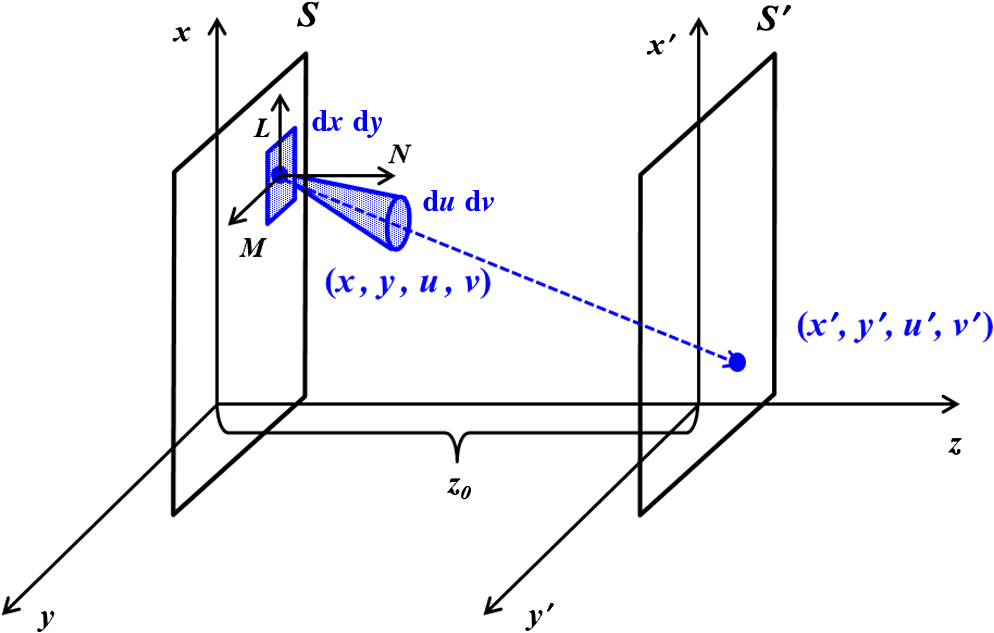
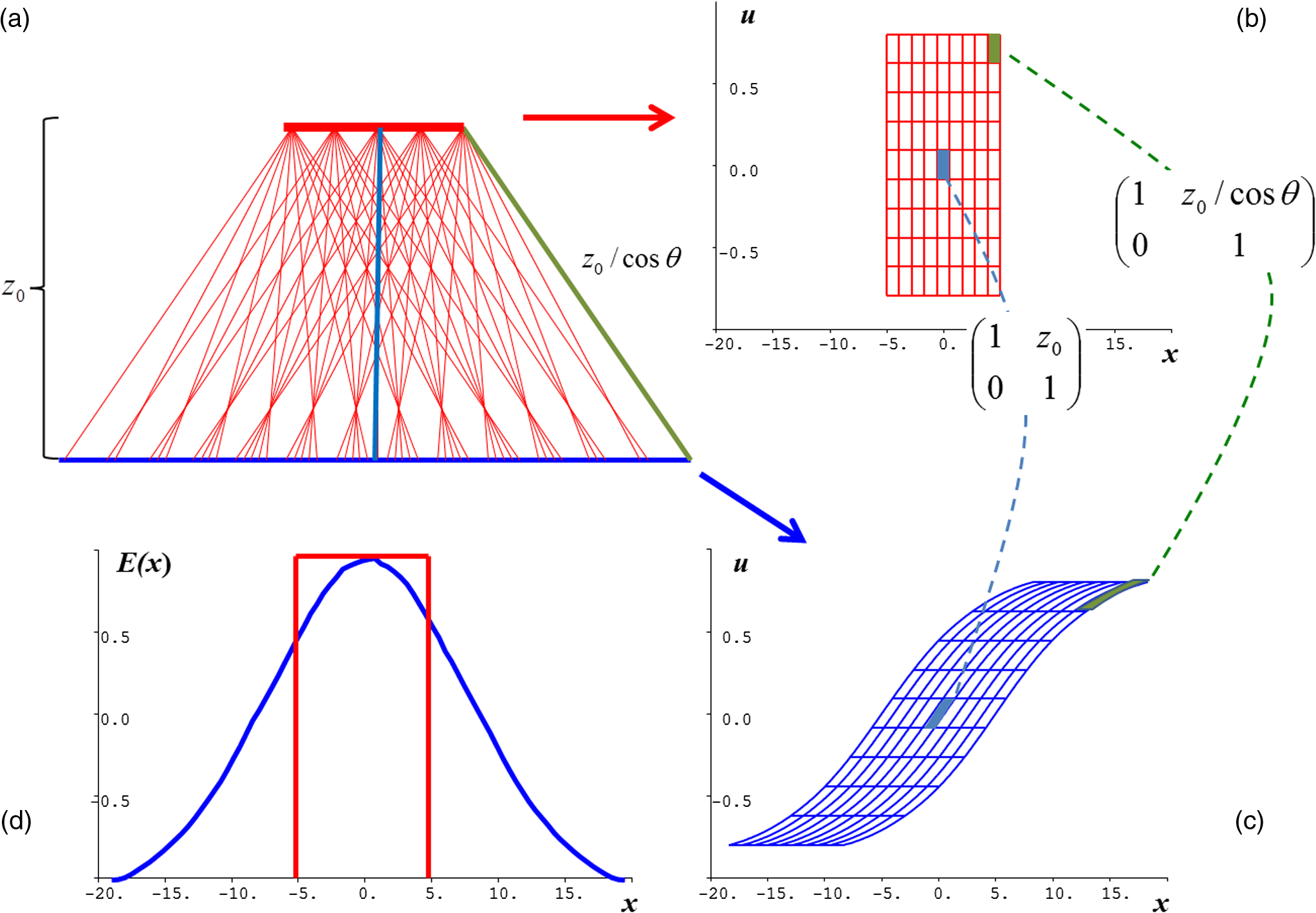
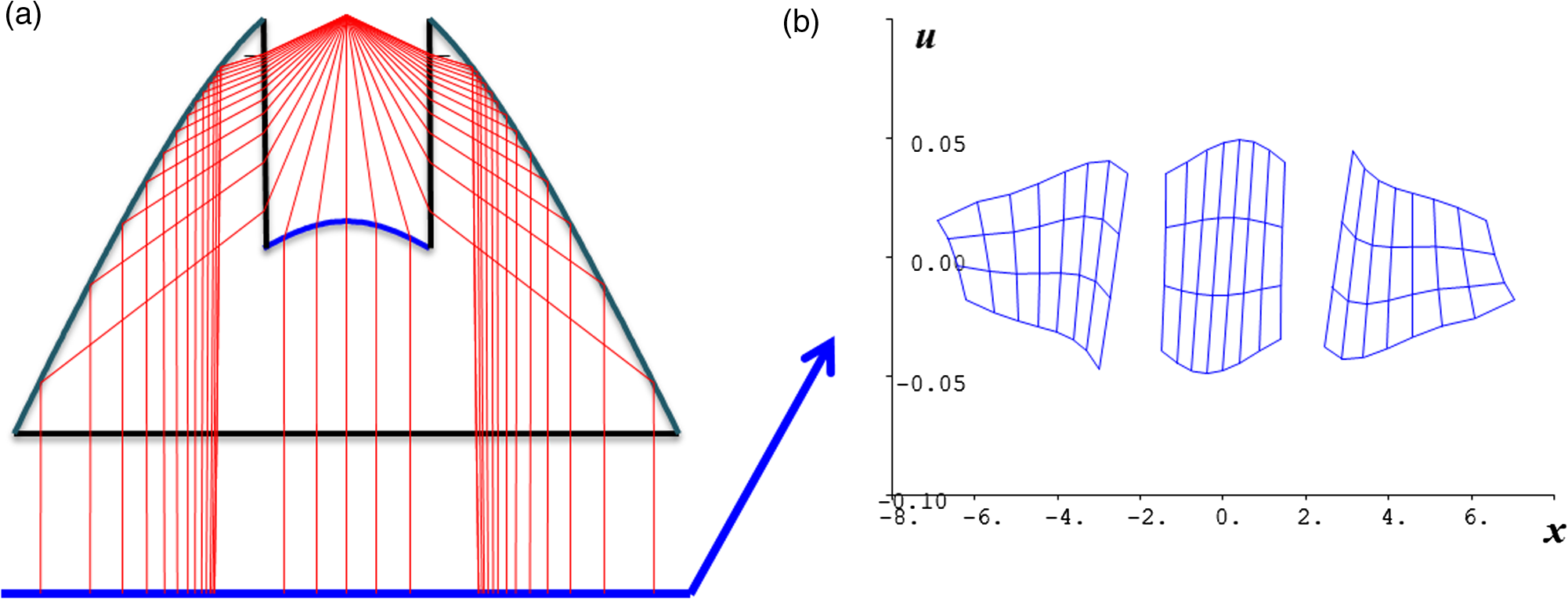
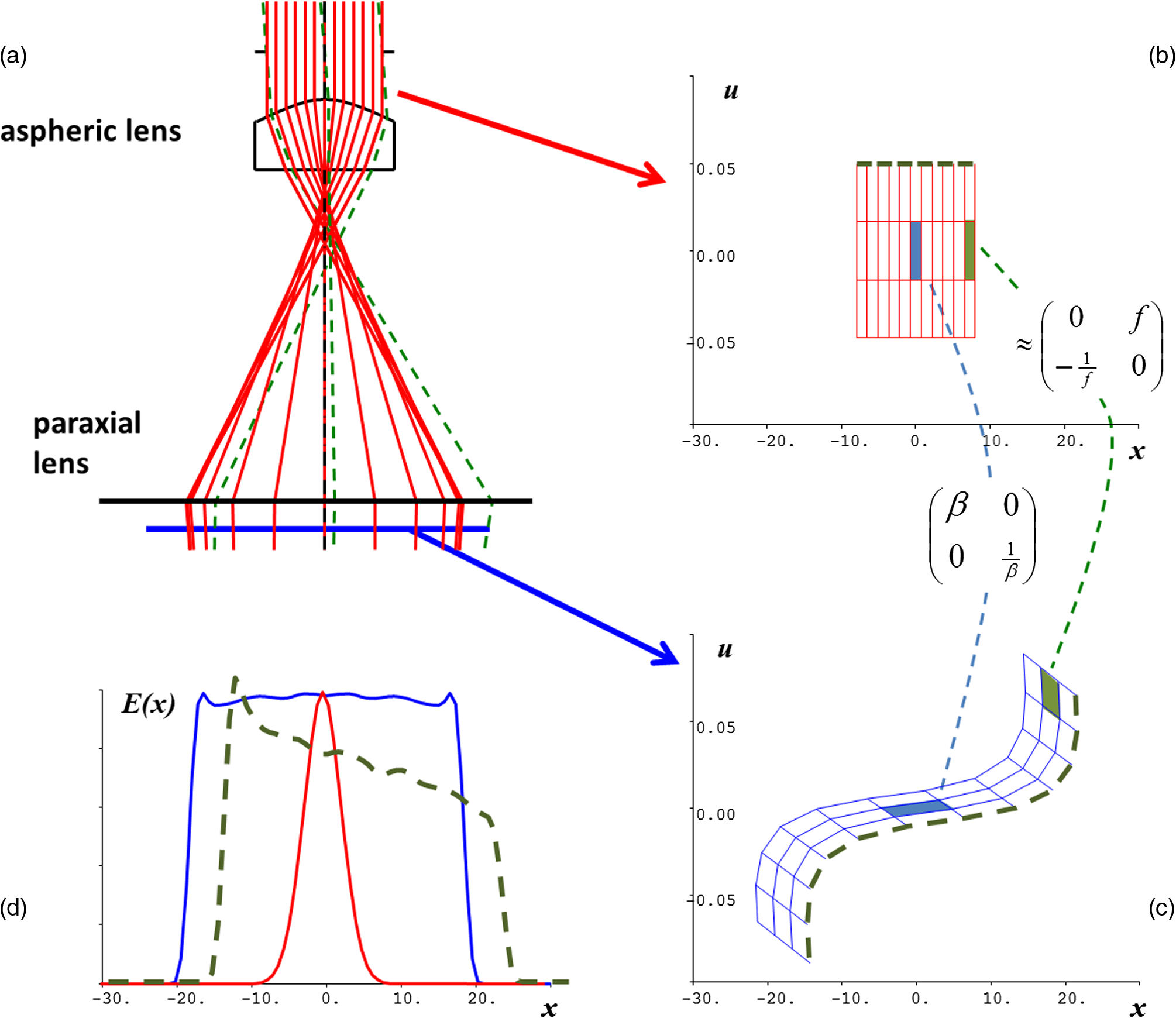
1.

Introduction

The basic design task in illumination design is the creation of a specified irradiance profile at a target plane.¹ In ideal lossless systems, all of the radiant flux of the light source shall be used; therefore, the source shape and size are of crucial importance. During the design of illumination systems, it is quite common to have idealized assumptions about the light source. Very often, nonphysical light sources, such as point sources, or perfectly collimated laser beams are assumed, since this idealization allows for the application of mathematical construction methods² for the illumination elements. For example, point sources quite naturally lead to conic reflector geometries, since they allow for perfect point-to-point transfer. Also, elements for more complex irradiance patterns can be constructed by mathematical equations, mapping, or beam-shaping algorithms.^3–5 Common examples are Gauss-to-top-hat beam shapers or freeform illumination reflectors for various applications.^6,7

However, real-world physical light sources exhibit a finite area–angle product, corresponding to a finite etendue. Light-emitting diodes in particular exhibit a large etendue due to their extended emission area and Lambertian intensity pattern, which needs to be considered during illumination design.^8,9 Solar applications, especially concentrators, are limited by the size of the sun. Lasers, especially poor quality lasers or lasers with pointing tolerances, have nonvanishing etendue, which needs to be considered. Currently, the finite etendue of the light sources is very often considered as a correction step during illumination design.¹⁰ That is, the system is laid out with a point-like light source and later the effect of finite source etendue is considered. Such methods have led to feedback methods in designing collimators.^11,12 Unfortunately, this iterative process lacks a deeper understanding of the effect of the source extensions, and fundamental implications and limitations in particular are not well defined. Therefore, a deterministic design process for extended sources is not yet available.

The approach within this paper is to take into account the etendue of the source from the very beginning. To do so, the method of phase space in optics is employed, which allows for a direct visualization of the etendue and radiance distribution.^13–15 There have already been attempts to illustrate the behavior of illumination systems in phase space, and they have proven to be helpful. However, in many references, this picture is limited to a conceptual or paraxial study. Within this work, we will try to extend this approach to a higher engineering level by a more sophisticated analysis of nonparaxial situations. In particular, we will show that the nonlinear transformations of phase space reveal basic limitations and properties of illumination systems. This analysis also allows for first attempts to design illumination systems that fully take into account the source etendue information.

2.

Introduction to Phase Space

2.1.

Concept of Phase Space

As we are dealing with illumination problems, we need to understand the basic connection of radiometry¹⁶ and phase space.^17,18 Let us consider a differential planar source element, or generally a radiation field, of a certain area $\mathrm{d}A$ radiating into some solid angle $\mathrm{d}\mathrm{\Omega }$. The related etendue element $\mathrm{d}H$ of this radiation field is defined as

Eq. (1)

$$\mathrm{d}H=n^2\times \mathrm{d}A\times \cos \theta \times \mathrm{d}\mathrm{\Omega }=\mathrm{d}x\times \mathrm{d}y\times \mathrm{d}u\times \mathrm{d}v,$$

where $n$ is the index of refraction, $\mathrm{d}A$ is the surface element, and $\cos (\theta )$ $\mathrm{d}\mathrm{\Omega }$ is the differential projected solid angle. If the radiation field (or source) is located in the $x/y$-plane and the normalized direction vector $(L,M,N)$ represents the direction of the solid angle element, as illustrated in Fig. 1, then the etendue is conveniently expressed in terms of differential area $\mathrm{d}A=\mathrm{d}x\times \mathrm{d}y$ and the projected solid angle element $\mathrm{d}u\times \mathrm{d}v$, where $u=n\times L$ and $v=n\times M$, as given in the right-hand side of Eq. (1).

Fig. 1

Illustration of the general radiance propagation in between parallel reference planes.

The amount of flux, or optical power, $d\varphi$ contained inside this differential etendue element defines the local radiance $L$ as

Eq. (2)

$$L(x,y,u,v)=\frac{\mathrm{d}\phi (x,y,u,v)}{\mathrm{d}x\times \mathrm{d}y\times \mathrm{d}u\times \mathrm{d}v}.$$

Therefore, in general, the radiance distribution is a four-dimensional function of the variables $(x,y,u,v)$. These four variables can be associated with the position and direction of a reference ray at a corresponding plane, as illustrated in Fig. 1.

Since four dimensions are very hard to visualize, we will restrict ourselves to two dimensions (as do most books on phase space). In other words, we will only consider light distributions or ray patterns in the $xz$-plane, such that any ray $r$ corresponds to a pair of $xu$-values, where the angular variable $u$ is associated with the angle $u=n\times \sin \theta$ of a ray relative to optical axis.

An illustration of several reference rays, or areas, in a $xu$-diagram is called a phase space diagram and defines the concept of phase space in optics. Following from Eq. (2), the radiance in the two-dimensional case is associated with an area in phase space

Eq. (3)

$$L(x,u)=\frac{\mathrm{d}\phi (x,u)}{\mathrm{d}x\times \mathrm{d}u}\approx \frac{\mathrm{\Delta }\phi (x,y)}{\mathrm{\Delta }x\times \mathrm{\Delta }u}.$$

From the radiance distribution, all other radiometric quantities, such as irradiance $E(x)$ and radiant intensity $I(u)$, can be calculated from a simple projection of the radiance distribution, as illustrated in Fig. 2. Moreover, for paraxial angles, the transformation properties of the rays and the radiance distribution are closely related to the ABCD-matrix formalism, which corresponds to a linear transformation within phase space, since

Eq. (4)

$$r^{\prime }=\left(\begin{array}{c}{x}^{\prime }\\ u^{\prime }\end{array}\right)=\left(\begin{array}{cc}A& B\\ C& D\end{array}\right)·\left(\begin{array}{c}x\\ u\end{array}\right)=M·r.$$

Any linear matrix operation $M$ in phase space corresponds to a general shear (or rotation) of the radiance distribution, as also illustrated in Fig. 2.

Fig. 2

Illustration of the general properties and relations in phase space: (a) illustrates a one-dimensional light source of angular and spatial extension $\mathrm{\Delta }u\mathrm{\Delta }x$, (b) is the corresponding radiance distribution in phase space, and (c) is the irradiance distribution resulting from integration along the angles.

2.2.

Quantization of Phase Space and Reference Rays

For a general extended light source, the radiance distribution can be separated into phase space areas/elements $A_i$. The flux contained in each element is simply related to the radiance distribution as

Eq. (5)

$${\phi }_i={\int }_{A_i}L(x,u)\times \mathrm{d}x\times \mathrm{d}u.$$

For further visualization and optimization within this paper, it is advantageous to split the phase space into small elements $A_i$ of either equal size or equal flux. In the special case of a Lambertian source ($L=\mathrm{const}.$), a particular simple case appears, since then the area is directly proportional to the flux

Eq. (6)

$${\phi }_i^{\text{Lambert}}=L_0·{\int }_{A_i}\mathrm{d}x\times \mathrm{d}u.$$

In this case, we can simply split the phase space into equal areas, and each element will carry the same amount of flux. Moreover, we can associate a reference ray $r_i$ with each phase space/flux element. Following this picture, we may now study the propagation of the phase space distribution. Throughout this paper, we will consider the transformation properties of these reference rays and the corresponding reference grid through an optical system. For a single point in phase space, this basically corresponds to a ray tracing from the source to the target. However, to predict radiance distributions, we also need to consider the transformation of the associated etendue area, i.e., the transformation of the phase space grid. As a simple example, we consider the free propagation of a Lambertian light source with large divergence, as illustrated in Fig. 3.

Fig. 3

Illustration of the free nonparaxial radiance propagation: (a) ray tracing illustration from source to detector, (b) and (c) radiance of the source and on the target plane, and (d) irradiance distribution at the source and target plane.

3.

Application Examples

We will now illustrate more complex examples of the phase space transformation for various optical systems. The local ABCD-matrixes can be calculated numerically; however, we will report and employ the approximate analytical shape of the matrix for better interpretation of the result.

3.1.

Parabolic Reflector

Let us consider a parabolic reflector in combination with an extended source. Figure 4 shows a situation where a source of 1-mm diameter is placed at the focus of the parabolic mirror (vertex-radius $R=20\mathrm{mm}$ and conic constant $k=-1$). The figure illustrates the transformation properties of this system form the source plane to an output plane at 17-mm distance to the mirror vertex. As the source is located in the front focal plane of the system and the image plane is (approximately) in the back focal plane, the basic phase space transformation corresponds to a $2f$-system, resulting in a 90-deg rotation in phase space (position is transformed to angles and vice versa). However, for large source angles, this transformation is nonuniform, meaning that the focal length varies across the parabola. For small angles (rays close to the vertex), the focal length is $f_0=10$, whereas for larger angles (e.g., 60 deg), we find, due to trigonometric relations, a larger focal length $f_1$. Therefore, the local phase space transformation corresponds to different scaling and focal length, respectively, at the edge of the parabolic as compared to the center. In consequence, the radiance distribution is rotated and “compressed” in the center.

Fig. 4

Illustration of phase space mapping for a parabolic mirror: (a) ray tracing illustration, (b) and (c) radiance of the source and of the target plane, and (d) irradiance distribution at the source and target plane.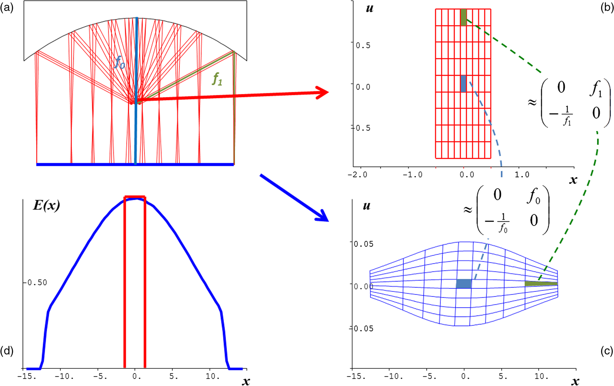

Since irradiance again corresponds to the projection of radiance distribution, and since we assumed a Lambertian source, the irradiance just corresponds to the diameter of the radiance distribution along the spatial dimension. This leads to an increased irradiance at the center of the output beam, as well-known for this type of illumination component, and illustrated in Fig. 4(d).

3.2.

Total Internal Reflection Reflectors

Another more complex example, resulting from combining the elements of a parabolic mirror and a lens, is a typical total internal reflection (TIR) collimator as illustrated in Fig. 5. The transformation again approximately corresponds to a rotation in phase space, if the source is at the focal spot of the lens or parabolic reflecting surface and if we consider a target plane approximately at the focal distance. In phase space, the central part (low angles) resembles the almost paraxial transformation of a lens, whereas the higher angles are reflected from the parabolic reflector part, leading to a similar distortion effect as for the parabola in Fig. 4. The full radiance distribution is separated in two distinct parts. The center part resembles the action of the lens, whereas the outer part corresponds to the nonlinear reflection at the parabolic. Since the local focal length near the center is shorter than at the edges, again a different scaling applies, leading to a smaller irradiance at the outside of the TIR-lens.

Fig. 5

Illustration of phase space mapping for a TIR-collimator: (a) ray tracing illustration and (b) radiance at the target plane for a 0.5-mm source.

3.3.

Gauss-to-Top-Hat Shaper

Let us now consider the well-known problem of shaping a Gaussian collimated laser beam into a top-hat from the perspective of phase space. Figure 6 illustrates a standard aspheric beam shaper, shaping a Gaussian input beam (full beam width 10 mm at $1/e^2$) to a top-hat beam (beam diameter 40 mm). For better visibility of the phase space transformation, we have added a paraxial lens at the target plane (only corresponding to a shear in angular direction). The resulting transformation of phase space is shown in Figs. 6(b) and 6(c). The input phase space grid in Fig. 6(b) corresponds to a $16\mathrm{mm}\times 0.1\mathrm{rad}$ ($\pm 3\mathrm{deg}$) section of the input phase space in front of the aspheric lens. However, in this example, the radiance is not equally distributed in that area, as in the examples before, but the beam has a Gaussian distribution, as illustrated in Fig. 6(d). So the flux in the phase space segments will be much larger in the middle. However, the equal phase space grid allows a visualization of the underlying transformation toward the target plan, as illustrated in Fig. 6(c). Obviously, the beam shaping is achieved by an approximate telescopic expansion at the center of the beam, distributing the flux into a larger area. At the edges of the beam, the input beam is almost focused, leading to a rotation and spatial compression of the input beam segment. In total, the phase space transformation is highly nonlinear. Only this nonlinearity across the beam (corresponding to a large variation of the local matrix $M$) allows a local beam expansion combined with a local beam focusing at the edge and thus the creation of the top-hat distribution.

Fig. 6

Illustration of phase space mapping for a beam shaper: (a) ray tracing illustration, (b) and (c) etendue mapping of the source and of the target plane, and (d) irradiance distribution at the source and target plane, the dashed line represents a laser tilted by 50 mrad.

4.

Illumination Design in Phase Space

Following up along the above analysis, we can transfer these findings into the design of illumination systems. Traditionally, the design of illumination systems is based either on strict mathematical construction methods or optimization based on statistical ray tracing, which requires a lot of computer time.

In contrast, we propose an alternate approach based on phase space. As discussed above, an illumination system can be analyzed quite accurately by a very limited number of reference rays and associated phase space patches. Tracing the reference rays results in the exact location of the radiance (irradiance) patches, whereas the surrounding local ABCD-transformation defines the shape of the radiance patch in phase space and the projection defines the irradiance contribution, respectively.

In consequence, we can optimize the position of the reference rays within the optical design to control the position where the flux patch will be deposited. And we can optimize the local ABCD-transformation, to control the shape of the phase space patch, and thus the local contribution to the irradiance.

Therefore, the general proposed design procedure is the following: first, we need to define an adequate number of reference rays and corresponding phase space patches. During design, we need to control the position of the reference rays and the ABDC-transformation properties, if we fully want to control the final radiance distribution. Controlling the ABCD-behavior can, for example, be achieved by controlling corner rays of a radiance patch. So the optimization can be done in any commercial design software.

As an example, let us again consider the Gauss-to-top-hat shaper mentioned previously. The single lens solution presented in Fig. 6 will produce a top-hat irradiance for a perfect collimated input beam. However, for a realistic “extended source” input beam (e.g., a low-quality laser beam or a laser with pointing errors), this design will create problems. If we, for example, simulate a pointing error of 0.05 rad, we find a distorted and shifted output beam profile, as illustrated in Fig. 6(d).

To optimize the design for such an extended source, we can now apply our method. Since we want to control radiance patches, reference rays for different angles and positions must be controlled. To achieve this, additional degrees of freedom are necessary. Therefore, we need to introduce an additional second aspheric lens, as shown in Fig. 7(a). Next, we need to define appropriate reference rays. For this example, we chose equidistant reference rays, marked by dots in Figs. 7(b) and 7(c). If we redistribute these reference rays at the target to have a deliberately distorted separation, we will obtain a top-hat distribution. In fact, this is the standard “mapping” design procedure for a shaper for an ideal collimated beam and will lead to a design similar to Fig. 6(a). However, if we now additionally control the local ABCD-transformation at the edges of the beam by aligning the reference rays corresponding to different input angles (here $\pm 0.05\mathrm{rad}$) to the same output position, as shown in Fig. 7(c), we find the optimized design shown in Fig. 7(a).

Fig. 7

Optimized version of a beam shaper: (a) ray tracing illustration, (b) and (c) corresponding phase space transformation of the source and at the target, illustrating the reference rays used for optimization, and (d) irradiance profile at the target, where the dashed line corresponds to a 50 mrad tilted laser beam.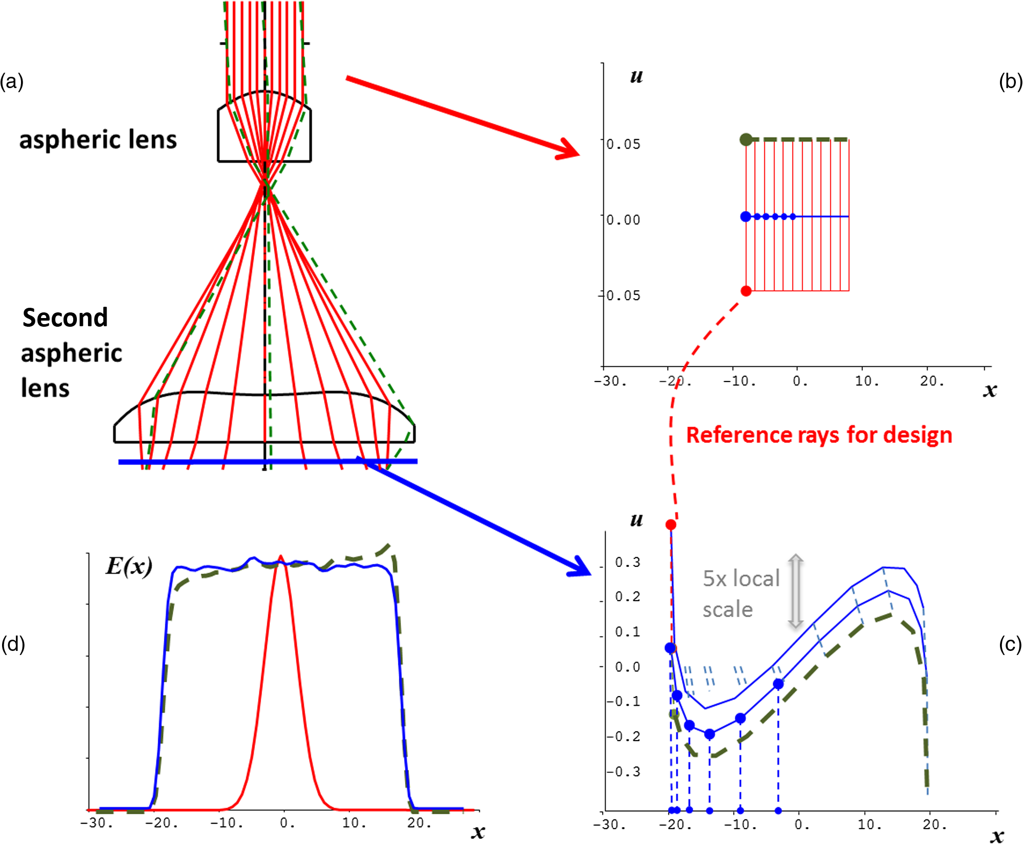

The advantages of this optimization are visible in Fig. 7(d), where we show the irradiance pattern at the target, for a collimated Gaussian input beam (solid lines) and for a tilted Gaussian input beam (dashed lines, for 0.05 rad tilt). Obviously, the optimized system preserves the shape and position of the top-hat profile also for the tilted beam. The main element to achieve this optimized system performance is the second highly aspheric lens, which images the stop onto the target at the edge of the beam and thus stabilizes the profile.

In summary, the phase space transformation in the new design is well controlled, to first spatially distort the radiance profile to form a top-hat and second to image the stop at the edge of the beam to stabilize it. Thus, the system is now optimized for an extended phase space region (corresponding to an extended source) and is therefore able to accept tilted laser beams or laser beams with large divergence.

5.

Conclusions

We have presented an alternate method to analyze illumination systems, which includes the etendue of a realistic extended source from the very beginning. An illustration of the radiance transformation properties in phase space allows intuitive and quantitative insight into the radiance and irradiance distribution at the exit of the system. The method allows a semianalytical analysis of the system behavior by determining the real ray tracing of reference rays in combination with an analysis of the local linear ABCD-properties. In consequence, the method allows considering the source extensions, source tolerances, and limitations in a very simple way. Moving forward, this also leads to design methods that are based on controlling reference rays and the transformation matrix.