1.

Introduction

2.

Optical Surface form Metrology Challenges

Is it more difficult to measure aspheres than spheres? The answer depends on the measurement device. Cartesian coordinate measurement machines, which measure the surface point by point, have a simple answer: No, there is no fundamental difference. As long as the gradients and size are comparable, the measurement principle does not take advantage of the high symmetry of spheres and therefore measures spheres and aspheres alike. Examples are the ISARA400 from IBSPrecision,⁸ the Panasonic UA3P instruments,⁹ or the NPMM200 developed at TU Ilmenau.¹⁰ However, they are comparatively slow, especially when high resolution areal measurements are required. Scanning measurements with a noncontact, optical probe increases the data acquisition rate and allows high data point densities along the scan path.

However, two problems arise when using optical probes on nonflat surfaces:

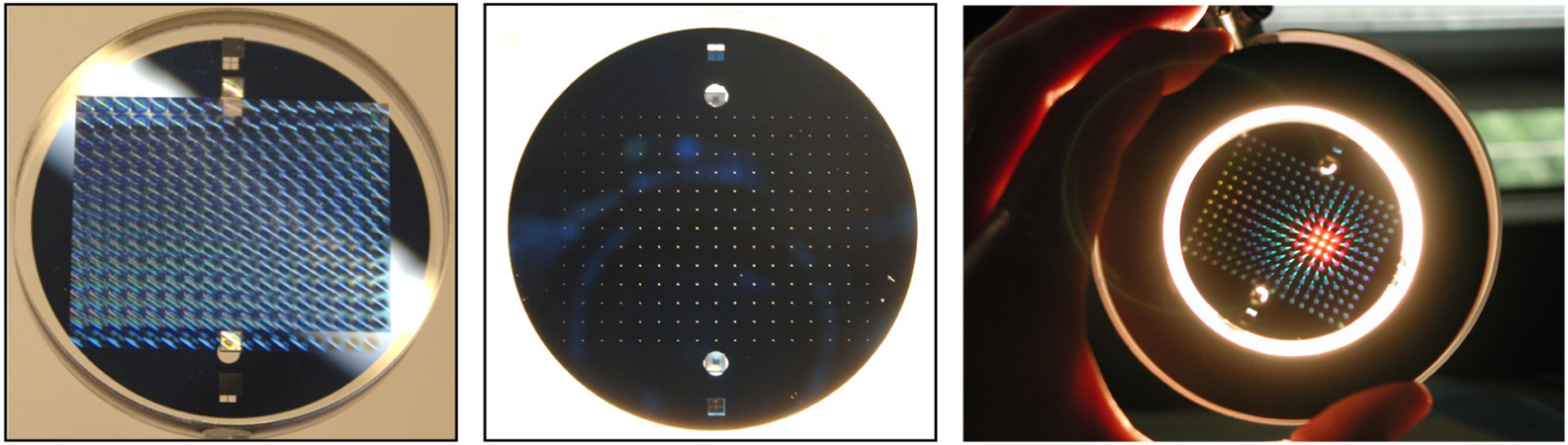
Both problems can be reduced if the probe and thus the angle of incidence of the measuring light are substantially perpendicular to the measured surface. For coordinate measuring machines, this normal incidence condition requires additional tilt axes or adapted coordinate measuring machines working in cylinder or even spherical coordinates. Examples are the MFU200 from Mahr,¹² the LuphoScan260 from Taylor-Hobson,¹³ or the NANOMEFOS¹⁴ at TNO. Exploiting the rotational symmetry of aspheres has an additional advantage: it allows faster scanning, reducing typical measurement times for measuring a centimeter-class SUT to 5 to 15 min for the fastest machines. Higher asphericities or a freeform shape again naturally violates the beneficial symmetry, so the deviations from sphericity or rotational symmetry at some point impose machine or sensor inherent limitations.

Due to the principle-inherent serial data acquisition of coordinate measuring machines, it is hard to achieve short measurement times in the subminute range as is desirable for fully automated production lines.

True areal measuring principles using CMOS or CCD detector arrays acquire millions of data points simultaneously. An example is the deflectometric measurement principle for specular surfaces.¹⁵ It measures the local gradient of the surface instead of the topography itself. The final shape is found by integration. It has been commercialized both as a point scanning method (e.g., by Trioptics¹⁶) or camera based as a full field method (e.g., by the company 3D-Shape¹⁷) and has found its application, e.g., in eye-glass testing but also as a method for testing focusing mirrors, e.g., in astronomy.¹⁸ There are other means of measuring the deflection of rays by the test surface or in transmission by a lens under test, e.g., phase shifting Schlieren.¹⁹ All deflectometric measurement approaches have in common that they are sensitive to gradients and thus excel in the detection of high-frequency surface defects even down to a height of a few nanometers. But for global shape measurements, due to the integration step involved, the absolute curvature and low-frequency surface errors tend to be detected with a lower accuracy, which is a disadvantage compared to height measuring methods such as interferometry.

Optical interferometry is a well-established and very sensitive method for the form measurement of aspheres.^20,21 To avoid both of the above-mentioned problems (retrace errors and vignetting), so-called compensation optics comes into play to compensate these departures and ensure normal or close-to-normal incidence of the testing light onto the SUT. State of the art is the use of computer generated holograms (CGH),^20–23 where the perfect shape of the asphere under test and typically also alignment aids are encoded in the CGH. The full field measurement then reveals the deviations from this perfect shape. The drawback of such holograms is, that for every design shape to be tested, a matching CGH has to be fabricated, which is costly and time consuming. To overcome this problem, flexible null optical systems have been suggested, e.g., based on adaptive optics.²⁴ Other technologies, such as sub-Nyquist interferometry,²⁵ multiple-wavelength-interferometry,²⁶ stitching,²⁷ or scanning²⁸ interferometry, also extend the flexibility of interferometric testing. Multiple-wavelength-interferometry has the advantage of absolute testing but like sub-Nyquist interferometry cannot solve the problem of vignetting. Stitching interferometry, e.g., with the ASI (Q) measurement station from QED,²⁹ is able to measure a wider range of aspheres with up to 1000 waves of departure from the best matching sphere without relying on dedicated, expensive null-optics. However, the surface has to be measured patch by patch in many time-sequential steps. To adjust the subaperture interferometer to every local patch, a high-precision and flexible multiaxial kinematics has to be implemented. Even though the number of patches can be reduced using a so-called variable optical null technology³⁰ that generates a wavefront that closely matches the local aspheric shape of each subaperture being measured, the measurement takes a couple of minutes up to hours depending on the number of subapertures. In the scanning interferometer Zygo Verfire asphere,²⁸ a relative movement between the asphere and the interferometer head along the optical axis results in null test ring zones that, combined together, reveal the SUT form. The principle works well for rotational symmetric surfaces but fails for general freeforms. A single measurement typically takes several minutes.

3.

Tilted Wave Interferometer

The tilted wave interferometer (TWI)^31,32 has been designed to meet the demand for very short measurement times while at the same time providing high precision and flexibility. These features are mainly achieved by a new illumination design³² in combination with a holistic calibration concept. It extends the single spherical wave front of a standard interferometer to an array of mutually tilted wavefronts. All of them simultaneously impinge onto the SUT. Thus for each area on the SUT, there is a fitting wave front that compensates the local deviation from the best fitting sphere, such that the laser light reaches the camera and produces interference fringes that contain the desired surface shape information. Since all wave fronts are there simultaneously, the SUT can be measured very quickly. In principle, the measurement time can be reduced to a single shot measurement. But in practice, it has proved advantageous to have four subsequent measurements with individual illumination settings to avoid overlapping of adjacent interferogram patches. Anyhow, the measurement time lies within a few seconds, while the allowable aspheric or freeform deviation from best fit sphere can be strong, of the order of several hundred micrometers.

Any setup that needs to measure surfaces with an accuracy better than a fraction of the wavelength relies on careful calibration, since at this nanometer accuracy level systematic errors from an imperfect setup are inevitable. A key factor of the TWI is an effective calibration concept.^33,34 It takes the common standard calibration from a two-dimensional (2-D) areal calibration to a volume calibration. This allows placing the SUT at any suitable position in front of the interferometer, which greatly enhances the flexibility of the instrument. It has been shown that this calibration concept can be generalized to other types of nonnull interferometric setups, too. In the next section, the setup and the calibration concept are briefly reviewed.

3.1.

TWI Implementation

Figure 1 shows how the tilted wave fronts are realized with the help of a matrix of point sources. The matrix of point sources consists of an especially designed microlens array that is followed by a pinhole array. Both parts together serve as point source array (PSA) for the test wavefronts (Fig. 2). The spherical wavefront from each point source is, after passing the beam splitter BS1, collimated by the lens C2 resulting in a set of plane wavefronts with different well-defined amounts of tilt. The tilted wavefronts are transformed to spherical wavefronts by the objective lens O to compensate the basic spherical form of the SUT. After reflection at the SUT, the wavefronts propagate back to the beam splitter BS1, where they are reflected to the camera arm of the interferometer. Here, the wavefronts coming from different parts of the SUT interfere with the reference wave, which is propagating along the reference arm. In the Fourier plane, an aperture stop A blocks all light that would generate fringes with a density that violates the Nyquist criterion. The generated composed interferogram (see Fig. 3) shows simultaneously all subapertures of the SUT with resolvable fringe density. Consequently, the complete SUT can be evaluated by a single coherent illumination without moving any component of the interferometer. However, to avoid crosstalk between adjacent patches, a four-step procedure is preferred that takes a few seconds longer. In this measurement scheme, only every second point source in each direction is activated simultaneously by a switchable sheet metal aperture array (AA in Fig. 1). The apertures in the array are spaced at twice the spacing of the point sources, blocking every second point source. To activate subsequently all sources, the aperture array merely needs to be moved laterally in $x$- and $y$-directions by one point source spacing distance. Note that the positions of the point sources themselves remain constant as they are defined by the monolithic PSA, so the movement of the aperture array does not influence the accuracy of the setup at all.

Fig. 1

Schematic setup of the interferometer with the central source and one exemplary off-axis source indicated. L, laser source; BS1, BS2, beam splitter; C1, C2, and C3, lens; PSA, point source array; AA, aperture array; M, mirror; O, objective; SUT, surfaces under test; A, aperture; IO, imaging optics; and C, camera.³³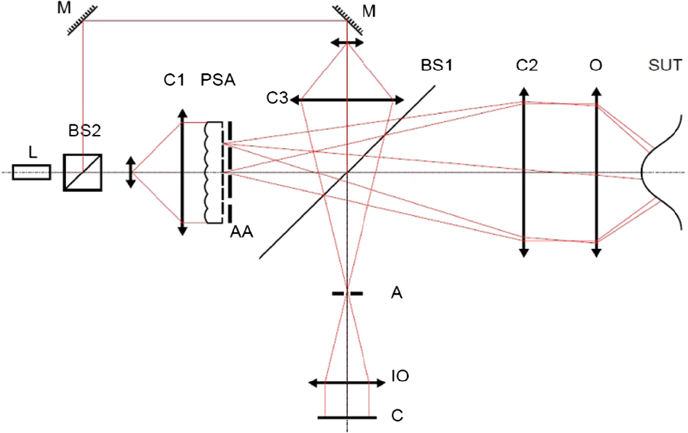

Fig. 2

PSA consisting of a microlens array followed by a pinhole array.

Fig. 3

(a) Composed interferogram showing all subapertures of the complete SUT with resolvable fringes; (b) four interferograms where only every second point source is activated.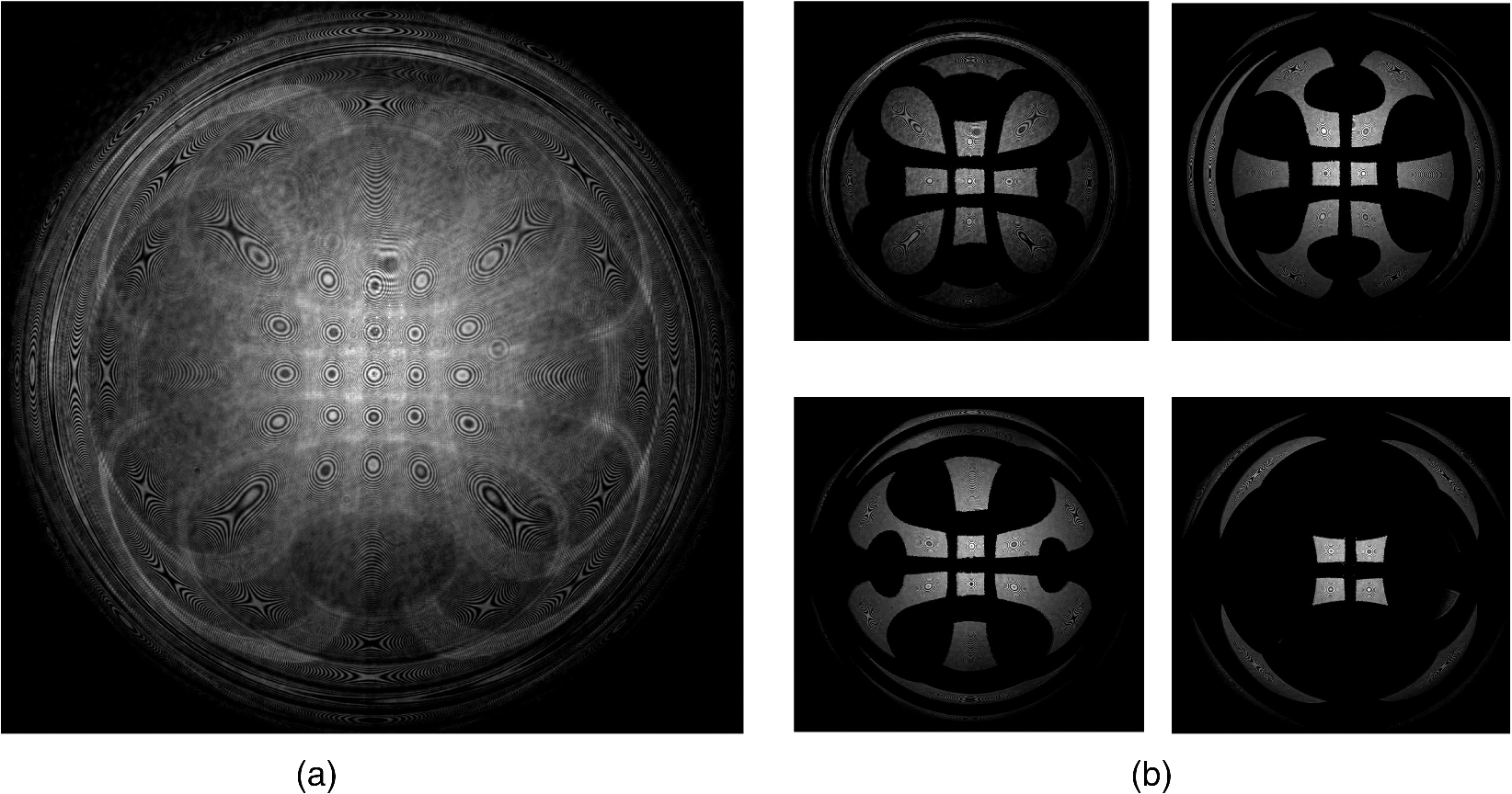

All tilted wave fronts propagate simultaneously through the interferometer along various ways, allowing an instantaneous measurement of the entire SUT.

Even though in the center of each interferogram patch, the fringe density is close to zero, the interferometer is no common-path arrangement. In a null-test configuration, a ray impinges perpendicularly on the surface and takes (after being reflected by the surface) the same path back through the interferometer. Therefore, it is sufficient in conventional setups to calibrate the OPD that is introduced by the interferometer for each pixel coordinate on the camera. The calibration can be expressed as a 2-D phase map $f=f(x,y)$ with $x$ and $y$ being the coordinates of the pixel and $f$ being some polynomial function or a look-up table containing the OPD correction value for each pixel. The intrinsic non-null setup requires a much more sophisticated calibration. In addition to the spatial dependency of the calibration function also field dependencies come into play: the ray impinges onto the surface under an angle that may differ from the perpendicular case and therefore the ray may take an arbitrary path through the interferometer, introducing retrace errors to the measurement. As a result, a 2-D calibration is not sufficient, since the introduced OPD also depends on the field angle, i.e., how the light passes through the setup. This can be described as a four-dimensional (4-D) dependency $f=f(x,y,m,n)$, where two dimensions ($x$ and $y$) cover the spatial dependency of the phase, as in the null-test example and the other two dimensions ($m$ and $n$) cover the field dependency. With such a 4-D description any possible ray through the system can be described. Details of the calibration procedure are given in Refs. 33 and 34. The evaluation of the interferogram needs some amount of computation power. It has been shown by Fortmeier et al. that important parts of the computation can be sped up by orders of magnitude using an analytical Jacobian approach.³⁵

4.

Measurement Results

One of the problems of precision metrology lies in the fact that the true shape of an artifact is not known to an arbitrary precision. Efforts are made to generate calibrated artifacts³⁶ that simplify the quantification of instrument’s measurement uncertainty. In this article, we show measurements of different instruments on the same artifacts. Such round robin testing on given samples, e.g., as organized in the past by UPOB e.V. and presented on their 10. Workshop 2016 Asphere Metrology on $8/9\mathrm{th}$ March, 2016, in Braunschweig, Germany,³⁷ does not give the absolute shape of the artifact but gives, in the deviations between the measurements, some insight into possible issues of the different measurement methods.

In our first round robin experiment, the measurement results of a weak asphere were compared between different machines, among them the ISARA400 by IBSPrecision and a TWI lab setup at ITO, University Stuttgart.³⁸ The geometry of the plastic sample can be seen in Fig. 4. The sample’s clear aperture is much smaller than its outer geometry. For the intercomparison, only the clear aperture was used, cut out from the measurement of the whole asphere.

Fig. 4

Weak asphere for intercomparison measurements.(a) Picture of the specimen and (b) raw phase image of the TWI lab setup measurement of the whole asphere.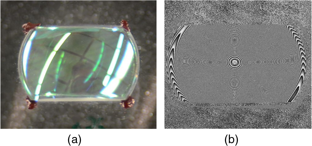

Figure 5 shows the measurements as deviation from design shape. The data of the TWI have been numerically interpolated to the measurement grid of the tactile instrument and the focus has been subtracted in both measurements.

Fig. 5

Comparison of measurements made by (a) a TWI lab setup and (b) a tactile instrument, the Isara400 by IBS Precision. The difference between the measurements (c) shows the good agreement of the measurements with some outliers that can be attributed to dust particles on the tactile probe.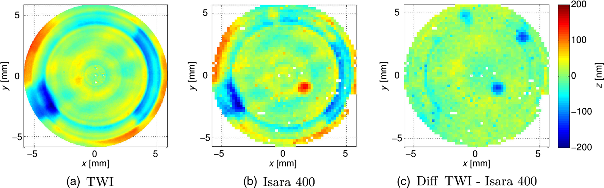

The major part of the difference can be attributed to outliers due to dust particles on the tactile probe. It is interesting to see that out of the three obvious outliers only one is easily seen in the measurement data and thus can be filtered, the other two somewhat hide in the topography deviation of the sample. The TWI data acquisition time for the sample was less than 1 min, while the tactile system, which, as a reference system, does not put the focus on measurement speed, had a measuring time in the hours region.

The results of another intercomparison of measurements among three instruments intended for integration into a production environment is given in Fig. 6. The measurement systems are two of interferometric type (Zygo Verifire Asphere, TWI) and one tactile (Panasonic UA3P). The specimen is a steep asphere with an aspheric deviation from best fit sphere of about 650 μm. It has been used for calibration of an MRF tool, so several MRF footprints are visible in its topography. The graphs show the deviation from design shape. The measurement times have been about 42 min on the UA3P, 8 min on the Verifire Asphere, and less than a minute on the TWI.

Fig. 6

Measurements of a steep asphere with about $650\text{-}\mu \mathrm{m}$ aspheric departure and several MRF testing footprints. Shown is the deviation from design, focus subtracted, measured on (a) TWI lab setup, (b) Panasonic UA3P, and (c) Zygo Verifire Asphere.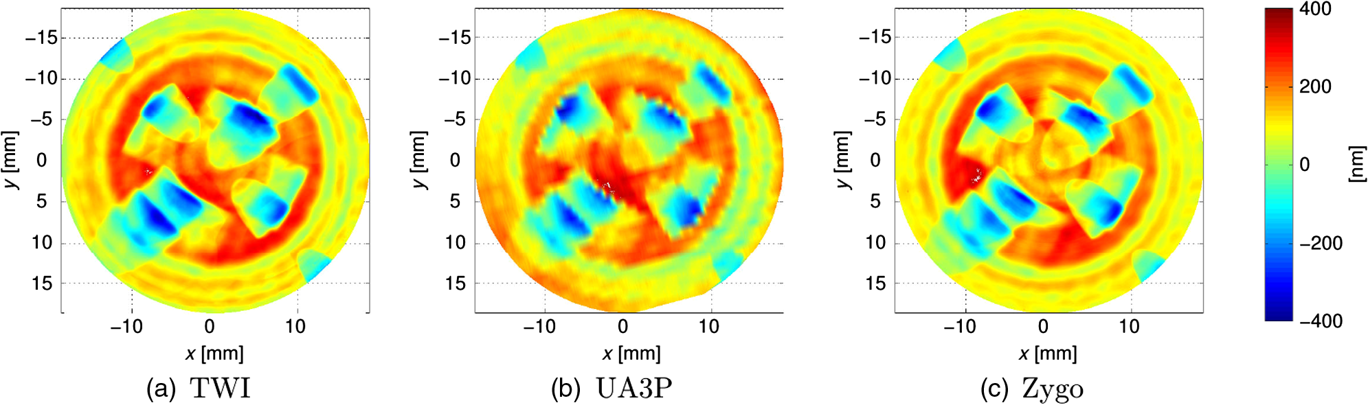

Fig. 7

Differences between the measurements of different instruments, (a) TWI lab setup–Panasonic UA3P, (b) TWI lab setup–Zygo Verifire Asphere, and (c) Zygo Verifire Asphere–Panasonic UA3P.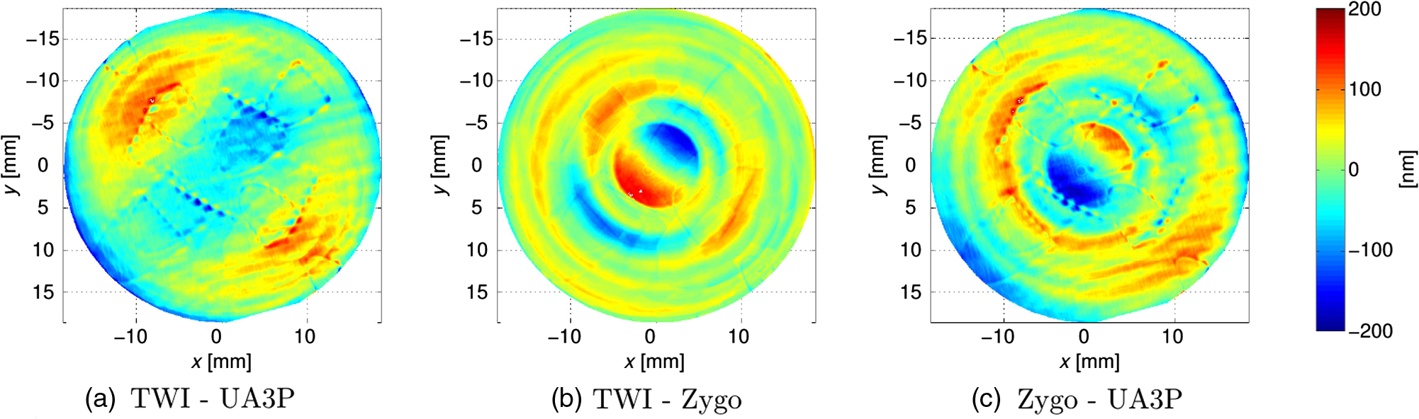

All measurements are similar and show the MRF footprints. For more detailed comparison, the results have been numerically aligned and interpolated to the data grid of the Zygo measurement and pairwise subtracted, see Fig. 7. Note that there are interpolation artifacts due to the low sampling of the tactile instrument. Even though at a first glance, the measurements seem very similar, the direct comparison shows some $\pm 150\mathrm{nm}$ (PV) deviations. The absolute real shape is not known; therefore, it is hard to attribute the differences to an individual instrument.

5.

Summary and Outlook

Asphere and freeform testing with short measurement time is possible with the proper illumination and calibration scheme. TWI combines the high accuracy and traceability of the interferometric principle with a high dynamic range of up to 10 deg max. gradient deviation from best fit sphere and up to 1.5 mm max aspheric departure from the best fitting spherical form without the need for compensation optics or moving the SUT. As in standard interferometers, the best fitting spherical shape is compensated with a spherical objective lens that defines the maximum diameter and radius of the SUT. The TWI implementation used in this paper uses 4-in. interferometer objective lenses for typical convex surfaces under test measuring several centimeters in diameter. Concave surfaces such as parabolic mirrors can be much bigger, even meter-class. TWI is able to measure both aspheres and freeforms. Furthermore it has—like all full field interferometric methods—a high lateral resolution across the full aperture (typically several hundred measurement points in diameter). An outstanding feature is its short data acquisition time ($\ll 1\min$), which is achieved by the highly parallelized data acquisition and which allows the integration into the workflow without unwanted delay in the processing chain. In principle, it is a single shot technique that allows the robust measurement of the entire surface in few seconds with no movement of the SUT, a height resolution better than 1 nm and a lateral resolution of typically several ten microns. The unique combination of these features makes the TWI a perfect candidate for the integration into the manufacturing workflow for aspheres and freeform production.

It has been shown by Fortmeier et al. in simulations that the absolute reconstruction of TWI can be further improved by adding an absolute path length, e.g., with a synthetic wavelength.³⁹ This will be the subject of future investigations. In this context, Fizeau-interferometry is advantageous. TWI on Fizeau-interferometers requires special attention that exactly one single reference wave is produced from the tilted wavefronts. Solutions have been proposed⁴⁰ and are currently under investigation.