Operator-based homogeneous coordinates: application in camera document scanning

Rigoberto Juarez-Salazar; Victor H. Díaz-Ramírez

doi:10.1117/1.OE.56.7.070801

27 July 2017 Operator-based homogeneous coordinates: application in camera document scanning

Rigoberto Juarez-Salazar, Victor H. Díaz-Ramírez

Author Affiliations +

Optical Engineering, Vol. 56, Issue 7, 070801 (July 2017). https://doi.org/10.1117/1.OE.56.7.070801

Abstract

An operator-based approach for the study of homogeneous coordinates and projective geometry is proposed. First, some basic geometrical concepts and properties of the operators are investigated in the one- and two-dimensional cases. Then, the pinhole camera model is derived, and a simple method for homography estimation and camera calibration is explained. The usefulness of the analyzed theoretical framework is exemplified by addressing the perspective correction problem for a camera document scanning application. Several experimental results are provided for illustrative purposes. The proposed approach is expected to provide practical insights for inexperienced students on camera calibration, computer vision, and optical metrology among others.

1. Introduction

Projective geometry is an important topic in computer vision because it provides a useful camera imaging model and its fundamental properties.¹ Some applications of this topic are found in camera motion,² camera calibration,³^,⁴ pose estimation for augmented reality,⁵ perspective correction,⁶ and three-dimensional (3-D) surface imaging⁷ among others.

Theoretical concepts of projective geometry are analyzed simply and elegantly using homogeneous coordinates.⁸^,⁹ However, projective geometry is commonly presented in abstract form, leaving a gap in how to apply it in computer vision problems.¹⁰ Moreover, homogeneous coordinates are used with a notation that masks basic geometrical aspects and may confuse the inexperienced readers.¹¹

In this paper, a simple and intuitive approach to expose some useful concepts of projective geometry is addressed. For this, an alternative notation for homogeneous coordinates based on operators is suggested. To highlight the relevance of this topic in computer vision, the presentation is motivated by a specific problem, namely the perspective correction for a “camera scanner” application.

First, the proposed operators for homogeneous coordinates are defined in Sec. 2. Next, some basic concepts of projective geometry in the one- (1-D) and two-dimensional (2-D) cases are presented in Secs. 3 and 4, respectively. Then, the pinhole camera model is derived in Sec. 5. A perspective correction method, useful for camera document scanning, is described in Sec. 6. Finally, the conclusions of this work are given in Sec. 7. The paper is complemented with two appendices. Appendix A presents the direct linear transformation method for homography matrix estimation. Finally, a simple method to obtain the camera parameters from homographies is explained in Appendix B.

2. Definition of Operators

2.1.

Operators $H$ and $S$

A point in an $n$ -dimensional space will be represented by a vector of the form

Eq. (1)

x = {[\begin{matrix} x_{1} & x_{2} & \dots & x_{n} \end{matrix}]}^{T},

where

{[\cdot]}^{T}

denotes the transpose. The homogeneous coordinates of the point are obtained by adding an extra entry to

x

with a value equal to the unity. The result is the

(n + 1)

-dimensional vector

Eq. (2)

H [x] = [\begin{matrix} x \\ 1 \end{matrix}],

where

H

will be referred to as the homogeneous operator.

The last entry of a homogeneous vector is known as the scale and will be recovered by the scale operator $S$ . This operator returns the last entry of any given vector. For instance, for the vectors in Eqs. (1) and (2), we have

Eq. (3)

x_{n} = S [x], and 1 = S [H [x]] .

The operator $H$ sets the scale to unity. Another operator that sets the scale to zero is needed. For this, we define the operator

Eq. (4)

H_{0} [x] = [\begin{matrix} x \\ 0 \end{matrix}] .

Note that the operator

H_{0}

does not affect neither the direction nor the norm of

x

. In projective geometry, the points represented by homogeneous coordinates of the form

Eq. (5)

H_{0} [x], x \neq 0_{n},

are known as ideal points, where

0_{n} = {[0, \dots, 0]}^{T}

is the

n

-dimensional zero vector.

The operators $H$ and $H_{0}$ can be considered as two particular cases of a more general operator defined as

Eq. (6)

H_{s} [x] = [\begin{matrix} x \\ s \end{matrix}],

where

s

is any scalar.

The procedure of adding an extra entry to vectors is reverted by returning the given vector except its last entry. For this, we define the inverse operator $H_{0}^{- 1}$ as follows. For any $(n + 1)$ -dimensional vector

Eq. (7)

y = {[\begin{matrix} y_{1} & y_{2} & \dots & y_{n} & y_{n + 1} \end{matrix}]}^{T},

the operator

H_{0}^{- 1}

is defined as

Eq. (8)

H_{0}^{- 1} [y] = {[\begin{matrix} y_{1} & y_{2} & \dots & y_{n} \end{matrix}]}^{T} .

Based on the operator

H_{0}^{- 1}

, the inverse of the operator

H_{s}

for

s \neq 0

is defined as

Eq. (9)

H_{s}^{- 1} [y] = \frac{s}{S [y]} H_{0}^{- 1} [y] .

In particular, the operator

H_{1}^{- 1}

(written simply as

H^{- 1}

) will be referred to as the inverse homogeneous operator.

The inverse $H_{0}^{- 1}$ is a linear operator. That is, for any two scalars $λ_{1}$ and $λ_{2}$ , we have

Eq. (10)

H_{0}^{- 1} [λ_{1} y_{1} + λ_{2} y_{2}] = λ_{1} H_{0}^{- 1} [y_{1}] + λ_{2} H_{0}^{- 1} [y_{2}] .

On the other hand, the operator

H_{s}^{- 1}

is invariant to nonzero scalar multiplication of its argument. That is,

Eq. (11)

H_{s}^{- 1} [λ y] = H_{s}^{- 1} [y], s, λ \neq 0 .

The operators

H_{s}

and

H_{s}^{- 1}

can be expressed in terms of the homogeneous operator and its inverse, namely

Eq. (12)

H_{s} [x] = Ξ_{s} H [x], and H_{s}^{- 1} [y] = H^{- 1} [Ξ_{s}^{- 1} y], s \neq 0,

where

Eq. (13)

Ξ_{s} = [\begin{matrix} I_{n} & 0_{n} \\ 0_{n}^{T} & s \end{matrix}],

and

I_{n}

being the

n \times n

identity matrix.

2.2.

Projection Operator $P$

In general terms, the homogeneous operator carries the representation of a point from $n$ - to $(n + 1)$ -dimensional vectors while the inverse homogeneous operator returns the representation from $(n + 1)$ - to $n$ -dimensional vectors. An important transformation emerges when, in the $(n + 1)$ -dimensional space, a linear mapping is applied. Mathematically, we describe this transformation by the projection operator defined as

Eq. (14)

P_{M} [x] = H^{- 1} [M H [x]],

where

M

is an

(n + 1) \times (n + 1)

matrix. A generalized version of the projection operator is obtained using

H_{s}

and its inverse as

Eq. (15)

P_{M, s} [x] = H_{s}^{- 1} [M H_{s} [x]] .

From Eq. (11), it follows that, for

s \neq 0

, the operator

P_{M, s}

is invariant to nonzero scalar multiplication of the matrix

M

; that is

Eq. (16)

P_{λ M, s} [x] = P_{M, s} [x], s, λ \neq 0 .

Let

b = P_{M, s} [a]

with

M

being a nonsingular matrix. From Eq. (15), we have that

a = H_{s}^{- 1} [M^{- 1} H_{s} [b]]

. Therefore, the inverse operator

P_{M, s}^{- 1}

is given by

Eq. (17)

P_{M, s}^{- 1} [x] = P_{M^{- 1}, s} [x], \det M \neq 0,

where

\det M

denotes the determinant of

M

.

Using the equations in Eq. (12), the operator $P_{M, s}$ can be expressed in terms of the projection operator, namely

Eq. (18)

P_{M, s} [x] = P_{Ξ_{s}^{- 1} M Ξ_{s}} [x], s \neq 0 .

Note that

M

and

Ξ_{s}^{- 1} M Ξ_{s}

are similar matrices. Some useful equalities of the defined operators are summarized in Table 1. For a more comprehensible reading of this paper, the reader is encouraged to demonstrate all the equalities in Table 1.

Table 1

Some useful equalities of the operators S, Hs, and PM,s. In all cases, we consider λ≠0, γ1 and γ2 are any scalars, x is a n-dimensional vector as given in Eq. (1), Ξs is the matrix defined in Eq. (13), y=λHs[x], M is a matrix of size (n+1)×(n+1), and W is a matrix of size m×(n+1).

Property	Description
(P1)	$H_{s}^{- 1} [H_{s} [x]] = x$	$s \neq 0$
(P2)	$H_{s} [H_{s}^{- 1} [y]] = \frac{s}{S [y]} y$	$s \neq 0$
(P3)	$x = H_{s}^{- 1} [y] \leftrightarrow \frac{S [y]}{s} H_{s} [x] = y$	$s \neq 0$
(P4)	$H_{s} [λ x] = λ H_{s / λ} [x]$
(P5)	$λ H_{s} [x] = H_{λ s} [λ x]$
(P6)	$H_{s} [W H_{s} [x]] = [\begin{matrix} W \\ H {[0_{n}]}^{T} \end{matrix}] H_{s} [x]$
(P7)	$H_{s} [x_{1} \pm x_{2}] = H_{s_{1}} [x_{1}] \pm H_{s_{2}} [x_{2}]$	$s_{1} \pm s_{2} = s$
(P8)	$H_{s}^{- 1} [λ y] = H_{s}^{- 1} [y]$	$s \neq 0$
(P9)	$λ H_{s}^{- 1} [y] = H_{λ s}^{- 1} [y]$	$s \neq 0$
(P10)	$H_{0}^{- 1} [γ_{1} y_{1} + γ_{2} y_{2}] = γ_{1} H_{0}^{- 1} [y_{1}] + γ_{2} H_{0}^{- 1} [y_{2}]$
(P11)	$S [γ_{1} x_{1} + γ_{2} x_{2}] = γ_{1} S [x_{1}] + γ_{2} S [x_{2}]$
(P12)	$H_{s}^{- 1} [y_{1} + y_{2}] = \frac{1}{S [y_{1} + y_{2}]} (S [y_{1}] H_{s}^{- 1} [y_{1}] + S [y_{2}] H_{s}^{- 1} [y_{2}])$	$s \neq 0$
(P13)	$H_{s}^{- 1} [y_{1} + y_{2}] - H_{s}^{- 1} [y_{1}] = \frac{S [y_{2}]}{S [y_{1} + y_{2}]} (H_{s}^{- 1} [y_{2}] - H_{s}^{- 1} [y_{1}])$	$s \neq 0$
(P14)	$H_{s} [x] = Ξ_{s} H [x]$
(P15)	$H_{s}^{- 1} [y] = H^{- 1} [Ξ_{s}^{- 1} y]$	$s \neq 0$
(P16)	$P_{λ M, s} [x] = P_{M, s} [x]$	$s \neq 0$
(P17)	$P_{M, s}^{- 1} [x] = P_{M^{- 1}, s} [x]$	$\det M \neq 0$
(P18)	$x_{2} = P_{M, s} [x_{1}] \leftrightarrow P_{M^{- 1}, s} [x_{2}] = x_{1}$	$\det M \neq 0$
(P19)	$P_{M, s} [λ x] = λ P_{M, s / λ} [x]$
(P20)	$λ P_{M, s} [x] = P_{M, λ s} [λ x]$
(P21)	$P_{M_{2}, s} [P_{M_{1}, s} [x]] = P_{M_{2} M_{1}, s} [x]$
(P22)	$P_{I_{n}, s} [x] = x$
(P23)	$P_{M, s} [x] = P_{Ξ_{s}^{- 1} M Ξ_{s}} [x]$	$s \neq 0$
(P24)	$H_{s} [P_{M, s} [x]] = \frac{s}{S [M H [x]]} M H [x]$	$s \neq 0$
(P25)	$P_{M, s} [H_{s}^{- 1} [y]] = H_{s}^{- 1} [M y]$	$s \neq 0$

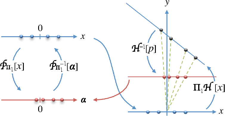
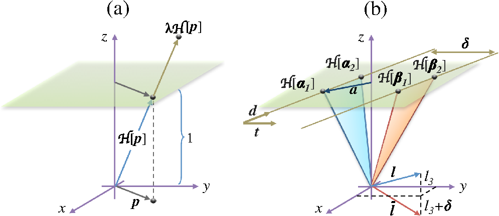
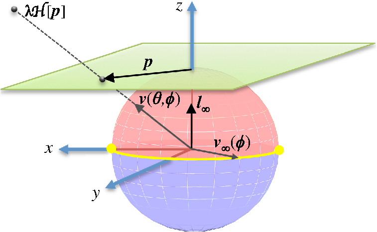
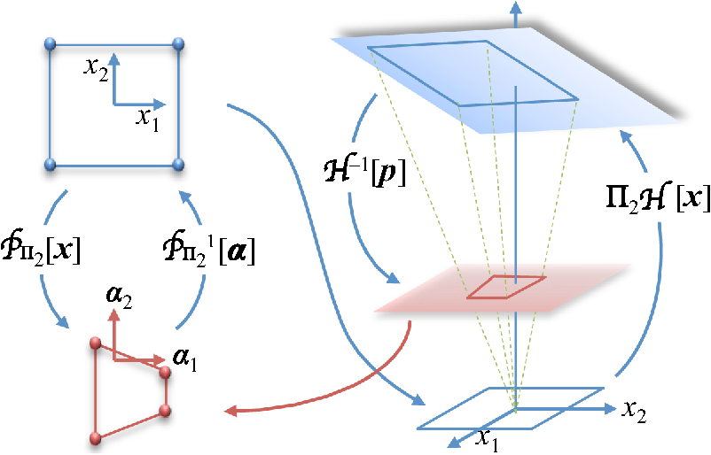
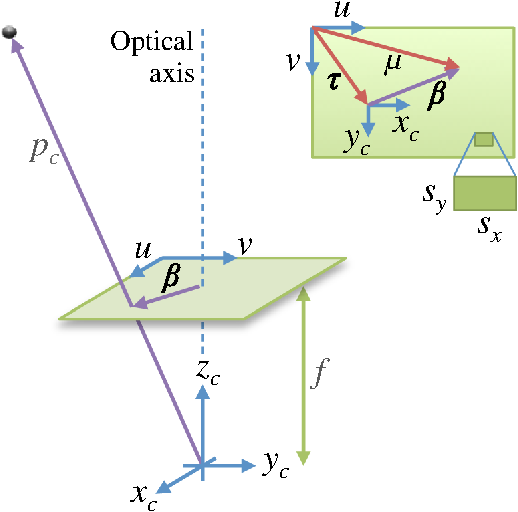
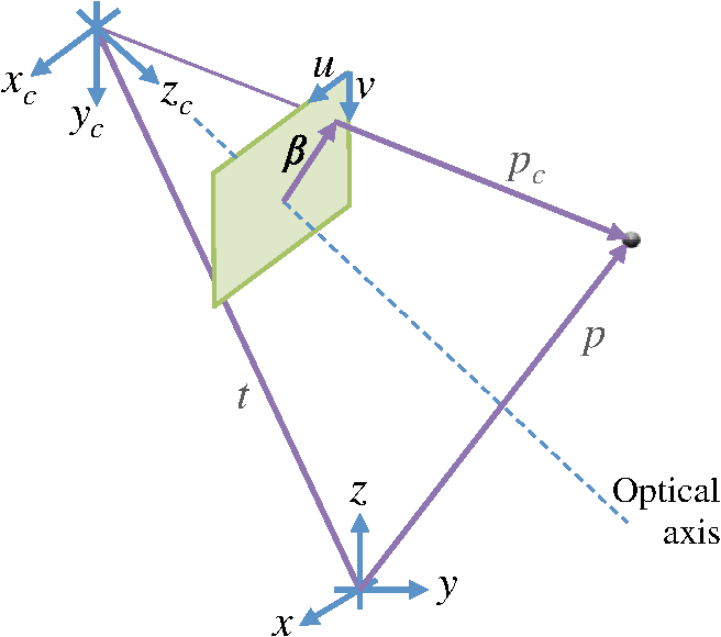
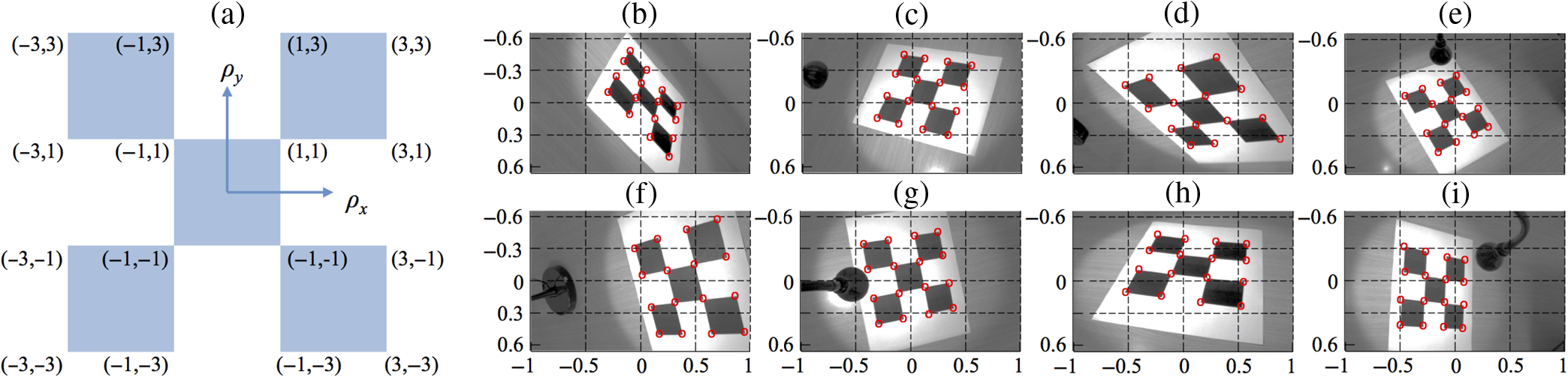
In the following sections, the defined operators are studied from an intuitive geometrical approach for the 1-D and 2-D cases. Then, the usefulness of this theoretical framework is illustrated by addressing the perspective correction problem for camera document scanning.

3. One-Dimensional Space

The 1-D real space can be represented as a line as shown in Fig. 1(a). In this space, a point at a finite distance from the origin is represented by a real number $x$ ; otherwise, the point is represented by the symbol $\infty$ .

Fig. 1

(a) The real line as the 1-D Euclidean space. (b) The 1-D space represented by the projective line ( $y = 1$ ) in a 2-D Euclidean space.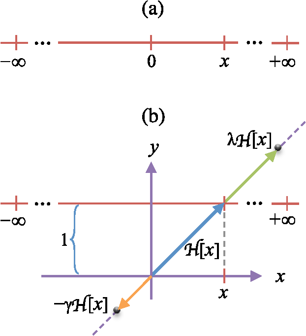

Alternatively, the 1-D space can be represented by the projective line $y = 1$ in the $x y$ -plane as shown in Fig. 1(b). Thus, the coordinate $x$ of a point in the line becomes the vector

Eq. (19)

y = H [x] = [\begin{matrix} x \\ 1 \end{matrix}] .

The coordinate

x

can be recovered from its homogeneous version

y

as the intersection between the line

y = 1

and the line with direction

H [x]

passing through the origin as shown in Fig. 1(b). This is described mathematically as

Eq. (20)

x = H^{- 1} [y] .

Note that the result is invariant to the scalar multiplication of

y

by a nonzero scalar [e.g.,

λ

and

- γ

as shown in Fig. 1(b)] because the intersection between lines is unaltered. In other words,

H^{- 1} [λ y] = H^{- 1} [- γ y] = H^{- 1} [y]

as stated by Eq. (11).

3.1.

Ideal Point

Homogeneous coordinates provide a different form to identify points of the real line. Consider the unit vector

Eq. (21)

u (θ) = [\begin{matrix} \sin θ \\ \cos θ \end{matrix}] .

Thus, the homogeneous representation of

x

given by Eq. (19) becomes

Eq. (22)

H [x] = λ u (θ),

where

λ^{2} = 1 + x^{2}

and

\tan θ = x

. From Eq. (22), we obtain

Eq. (23)

x = H^{- 1} [u (θ)] .

Since a vector

u

and its opposite

- u

represent the same point (i.e.,

H^{- 1} [u] = H^{- 1} [- u]

), all points of the real line at a finite distance from the origin are associated to a unique angle

θ

in the open interval

(- π / 2, π / 2)

; i.e., the vectors

u

different to [1, 0] and

[- 1,0]

in the quadrants I and II, as shown in Fig. 2.

Fig. 2

Representation of points of the real line using homogeneous coordinates. Opposite homogeneous vectors represent the same point; thus, there is a single point at infinity, given by 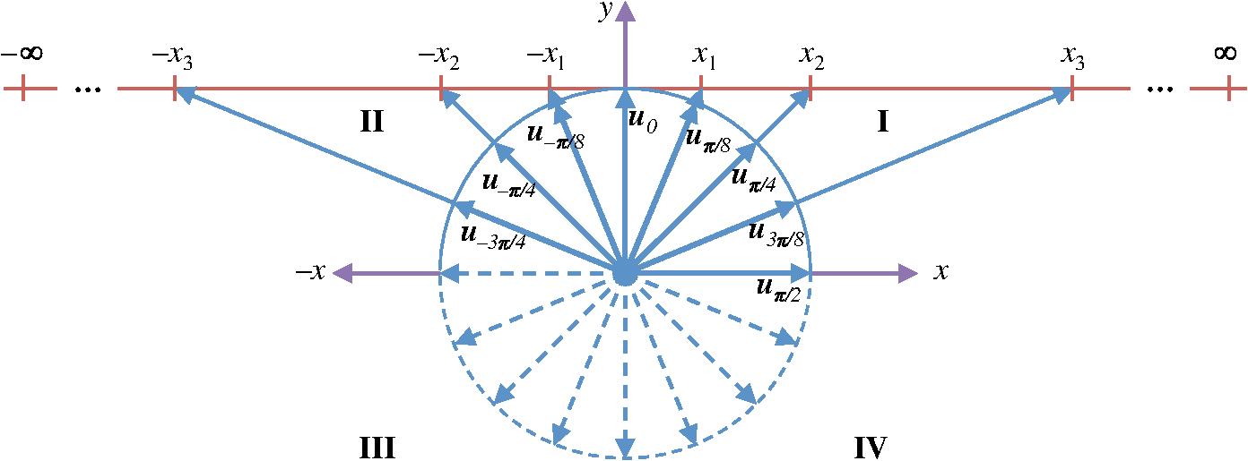$u (π / 2) = {[1,0]}^{T}$ .

Intuitively, the real line in Euclidean representation has two points at infinity, namely $- \infty$ and $+ \infty$ . However, in projective geometry, the real line has only a single point at infinity given by the homogeneous coordinates

Eq. (24)

ψ = [\begin{matrix} 1 \\ 0 \end{matrix}],

which is associated to

u (π / 2)

, as shown in Fig. 2. It could be argued that

π / 2

corresponds to

+ \infty

while

- π / 2

to

- \infty

. However, note that

u (- π / 2) = - ψ

is the opposite of

ψ

. Hence, they represent the same point.

Note that $H^{- 1} [ψ] = 1 / 0$ is consistent with the notion that $ψ$ represents a point at infinity distance from the origin. According to the concepts of projective geometry, the vector $ψ$ represents an ideal point, see Eq. (5).

3.2.

One-Dimensional Projection

The line $y = 0$ can be transformed to any other line by applying a rotation $Q = [q_{1}, q_{2}]$ and a translation $s$ . Thus, a point in the line $y = 0$ , represented by the scalar $x$ , becomes a point in the $x y$ -plane given by the vector

Eq. (25)

p = q H_{0} [x] + s = Π_{1} H [x],

where the matrix

Π_{1}

will be referred to as the reference line parameters and has the explicit form

Eq. (26)

Π_{1} = [\begin{matrix} q_{1} & s \end{matrix}] .

The first column of

Π_{1}

and the determinant

\det Π_{1}

provide the direction of the reference line and its distance from the origin, respectively.

If the matrix $Π_{1}$ is singular, the vectors $q_{1}$ and $s$ are collinear. In this case, the origin is a point of the transformed line (the distance of the line from the origin is zero). The matrix $Π_{1}$ is nonsingular when $q_{1}$ and $s$ are linearly independent. In this case, the origin is not a point of the transformed line.

Let $p$ in Eq. (25) be the homogeneous coordinates of a point $α$ in the line. Thus, we obtain the 1-D projection

Eq. (27)

α = H^{- 1} [p] = H^{- 1} [Π_{1} H [x]] = P_{Π_{1}} [x] .

The transformations by

P_{Π_{1}} [x]

and its inverse

P_{Π_{1}^{- 1}} [α]

are shown in Fig. 3.

Fig. 3

The 1-D projection.

4. Two-Dimensional Space

4.1.

Points and Lines in the Plane

Any point in the 2-D space can be represented as the vector

Eq. (28)

x = {[\begin{matrix} x_{1} & x_{2} \end{matrix}]}^{T} .

Moreover, the point

x

can be represented by its homogeneous coordinates

Eq. (29)

H [x] = [\begin{matrix} x \\ 1 \end{matrix}],

as shown in Fig. 4(a). Note that

H

takes the 2-D vector

x

(in the plane

z = 0

) and converts it to the 3-D vector

H [x]

, where

x

is unaltered but now it lies in the projective plane

z = 1

. It is worth mentioning that the vector

x

can be recovered from

λ H [x]

as the point of intersection of the line with points

0_{3}

and

λ H [x]

, see Eq. (11). That is,

Eq. (30)

x = H^{- 1} [λ H [x]], λ \neq 0 .

A line in the plane

x y

-plane can be written as the homogeneous equation

Eq. (31)

l_{1} x_{1} + l_{2} x_{2} + l_{3} = 0,

where

l_{1}

,

l_{2}

, and

l_{3}

are coefficients. Using homogeneous coordinates, Eq. (31) becomes

Eq. (32)

l^{T} H [x] = 0,

where

x = {[x_{1}, x_{2}]}^{T}

is a point of the line and

l = {[l_{1}, l_{2}, l_{3}]}^{T}

is the vector that defines the line. Equation (32) exhibits that

l

and

H [x]

are orthogonal vectors. Note that the vector

l

is unique up to scale, i.e., the vectors

l

and

λ l

, with

λ \neq 0

, represent the same line.

Fig. 4

(a) The 2-D space represented by the projective plane ( $z = 1$ ). (b) Parallel lines in the plane.

Let $x_{1}$ and $x_{2}$ be two different points in the $x y$ -plane. The vector $l$ of the line passing through $x_{1}$ and $x_{2}$ can be obtained by the cross product as

Eq. (33)

l = H [x_{1}] \times H [x_{2}] .

By definition of the cross product, the vector

l

is orthogonal to

H [x_{1}]

and

H [x_{2}]

. Therefore, these vectors satisfy Eq. (32).

Consider two lines defined by the vectors $l_{1}$ and $l_{2}$ . If $x$ is the intersection point of these lines, then $H [x]$ is orthogonal to $l_{1}$ and $l_{2}$ . That is

Eq. (34)

λ H [x] = l_{1} \times l_{2},

where

λ = S [l_{1} \times l_{2}]

. Therefore, the intersection point of the lines

l_{1}

and

l_{2}

is

Eq. (35)

x = H^{- 1} [l_{1} \times l_{2}] .

4.2.

Parallel Lines

Two different lines are parallel if its defining vectors are of the form

Eq. (36)

l = [\begin{matrix} l_{1} \\ l_{2} \\ l_{3} \end{matrix}], \bar{l} = λ [\begin{matrix} l_{1} \\ l_{2} \\ l_{3} + δ \end{matrix}],

where

λ

,

δ \neq 0

. This can be verified as follows. Consider two parallel lines in the plane with points

α

and

β

given, respectively, by

Eq. (37)

α = a + γ d, and β = a + γ d + δ t,

where

γ

is a parameter,

δ \neq 0

is a constant,

a

is a reference point,

d

is a unit vector with direction of the line, and

t

is a unit vector orthogonal to

d

, i.e.,

Eq. (38)

H_{0} [t] \times H_{0} [d] = H [0_{2}],

as shown in Fig. 4(b). Two points of each line are

α_{1} = a + γ_{1} d, β_{1} = a + {\bar{γ}}_{1} d + δ t, α_{2} = a + γ_{2} d, β_{2} = a + {\bar{γ}}_{2} d + δ t .

Thus, the vector of the line with points

α

is

Eq. (39)

l = H [α_{1}] \times H [α_{2}] = (γ_{2} - γ_{1}) H [a] \times H_{0} [d],

or, since the line is unaffected by scaling of its vector

Eq. (40)

l = H [a] \times H_{0} [d] .

Similarly, the vector of the line with points

β

is

Eq. (41)

\bar{l} = H [β_{1}] \times H [β_{2}] = ({\bar{γ}}_{2} - {\bar{γ}}_{1}) (l + δ H [0_{2}]) = λ (l + δ H [0_{2}]),

where

λ = {\bar{γ}}_{2} - {\bar{γ}}_{1}

. Therefore, the vectors

l

and

\bar{l}

given in Eq. (36) represent parallel lines.

It is worth mentioning that, if $l$ is the vector of a line with direction $d$ [see Eq. (40)], then the vector $H_{0}^{- 1} [l]$ is orthogonal to $d$ , namely

Eq. (42)

d^{T} H_{0}^{- 1} [l] = d^{T} H_{0}^{- 1} [H [a] \times H_{0} [d]] = H_{0} {[d]}^{T} (H [a] \times H_{0} [d]) = 0 .

4.3.

Ideal Points and the Line at Infinity

In the Euclidean geometry, two parallel lines in the plane do not intersect. However, in the projective geometry, two different lines always intersect at a point. Consider the parallel lines given by the vectors in Eq. (36). Using Eq. (35), the intersection point is

Eq. (43)

H^{- 1} [l \times \bar{l}] = H^{- 1} [H [0_{2}] \times l] = H^{- 1} [ψ],

where

Eq. (44)

ψ = {[\begin{matrix} - l_{2} & l_{1} & 0 \end{matrix}]}^{T}

is the point of intersection in homogeneous coordinates. Note that

H^{- 1} [ψ] = [- l_{2} / 0, l_{1} / 0]

provides the insight that parallel lines intersecting at a point at infinity. As in the 1-D case, the vector

ψ

represents ideal points, see Eq. (5).

The vector $ψ$ is associated with the direction $d$ of the line $l$ . This is verified by taking into account that $H_{0}^{- 1} [l]$ is orthogonal to $d$ [Eq. (42)] as well as to $H_{0}^{- 1} [ψ]$ ( $H_{0}^{- 1} {[ψ]}^{T} H_{0}^{- 1} [l] = 0$ ), then

Eq. (45)

H_{0}^{- 1} [ψ] = λ d,

where

λ

is some nonzero scalar.

All ideal points given by Eq. (44) are collinear. The vector of such a line, known as the line at infinity, is

Eq. (46)

l_{\infty} = H [0_{2}] = {[\begin{matrix} 0 & 0 & 1 \end{matrix}]}^{T} .

This can be easily verified by

l_{\infty}^{T} ψ = 0

as required by Eq. (32).

The ideal point $ψ$ in Eq. (44) was obtained as the intersection of two parallel lines $l$ and $\bar{l}$ . However, the intuition suggests that the same result could be obtained by computing the intersection of the line $l$ and the line at infinity $l_{\infty}$ . In fact, we have that

Eq. (47)

ψ = l \times l_{\infty} .

Thus, using Eq. (45), the direction

d

of any line

l

is given by

Eq. (48)

λ d = H_{0}^{- 1} [l \times l_{\infty}],

where

λ

is a nonzero scale factor. For this reason, the line

l_{\infty}

is interpreted as the set of directions of lines in the plane.

Similar to the 1-D case, homogeneous coordinates provide a different form to identify points of the plane. Consider the unit vector

Eq. (49)

v = {[\begin{matrix} \sin θ \cos ϕ & \sin θ \sin ϕ & \cos θ \end{matrix}]}^{T},

where

θ

and

ϕ

are polar and azimuth angles, respectively. Thus, the homogeneous coordinates for each point

x = {[x_{1}, x_{2}]}^{T}

on the plane are given by

Eq. (50)

H [x] = λ v,

where

λ^{2} = 1 + x_{1}^{2} + x_{2}^{2}

. From Eq. (50), the following relation holds

Eq. (51)

x = H^{- 1} [v (θ, ϕ)] .

The points of the plane at a finite distance from the origin are given by $v (θ, ϕ)$ with $θ \in [0, π / 2)$ and $ϕ \in [- π, π)$ , i.e., the upper hemisphere of the unit sphere, see Fig. 5. The points of the plane at infinity distance from the origin are parameterized by $θ = π / 2$ and $ϕ \in (- π / 2, π / 2]$ . These points have the homogeneous coordinates

Eq. (52)

v_{\infty} = {[\begin{matrix} \cos ϕ & \sin ϕ & 0 \end{matrix}]}^{T},

see Eq. (44). That is, the ideal points are represented by the half equator of the unit sphere, see yellow line in Fig. 5.

Fig. 5

Representation of points of the plane using homogeneous coordinates $v$ . The upper hemisphere represents points of the plane at a finite distance from the origin, and the half of the equator (yellow semicircle) represents points at infinity.

4.4.

Two-Dimensional Projection

Any plane in the 3-D space can be obtained as the plane $z = 0$ after a rotation $Q = [q_{1}, q_{2}, q_{3}]$ and a translation $s$ . Thus, the points represented by $x = {[x_{1}, x_{2}]}^{T}$ , becomes

Eq. (53)

p = Q H_{0} [x] + s = Π_{2} H [x],

where the matrix

Π_{2}

will be referred to as the reference plane parameters and has the explicit form

Eq. (54)

Π_{2} = [\begin{matrix} q_{1} & q_{2} & s \end{matrix}] .

The cross product of the first two columns of

Π_{2}

and

\det Π_{2}

provides the normal to the reference plane and its distance from the origin, respectively.

The matrix $Π_{2}$ is singular when $r_{1}$ , $r_{2}$ , and $t$ are coplanar. In this case, the origin $0_{3}$ is a point of the transformed plane (the distance of the reference plane from the origin is zero). Otherwise, $Π_{2}$ is a nonsingular.

Let $p$ in Eq. (53) be the homogeneous coordinates of a point $α$ in the projective plane. Thus, the relation between the points $α$ and $x$ is given by the 2-D projection $P_{Π_{2}}$ , namely

Eq. (55)

α = H^{- 1} [p] = H^{- 1} [Π_{2} H [x]] = P_{Π_{2}} [x] .

The projection

P_{Π_{2}} [x]

and its inverse

P_{Π_{2}^{- 1}} [α]

are shown in Fig. 6.

Fig. 6

The 2-D projection.

4.5.

Properties of the Two-Dimensional Projection

As shown in Fig. 6, the 2-D projection $P_{Π_{2}}$ excludes several geometrical properties; e.g., shape, angles, lengths, and ratio of lengths. Fortunately, there are some geometrical properties that are preserved. Particularly, we are interested in three of them that are very useful in practice: namely straightness, line–line intersection, and parallelism of the normal and line at infinity vectors.

4.5.1.

Straightness property

This property states that a 2-D projection transforms lines to lines.¹² This can be shown as follows. Consider a line with vector $l$ and points $x$ , that is

Eq. (56)

0 = l^{T} H [x] .

Next, the points

x

are transformed to

α

by Eq. (55). Solving Eq. (55) for

x

and substituting in Eq. (56), we obtain

Eq. (57)

0 = l^{T} H [P_{Π_{2}^{- 1}} [α]] = \frac{l^{T} Π_{2}^{- 1} H [α]}{S [Π_{2}^{- 1} H [α]]},

or

Eq. (58)

0 = m^{T} H [α],

where

Eq. (59)

m = Π_{2}^{- T} l,

with

Π_{2}^{- T}

being the abbreviation of

{(Π_{2}^{- 1})}^{T}

or

{(Π_{2}^{T})}^{- 1}

. In summary, the points

x

of a line

l

are transformed by

P_{Π_{2}}

to points

α

of a new line

m

.

4.5.2.

Line–line intersection

Preservation of the line–line intersection by a 2-D projection refers to the following. If

Eq. (60)

x_{0} = H^{- 1} [l_{1} \times l_{2}]

is the point where the lines

l_{1}

and

l_{2}

intersect, then

Eq. (61)

α_{0} = P_{Π_{2}} [x_{0}]

is the point where intersect the lines

Eq. (62)

m_{1} = Π_{2}^{- T} l_{1} and m_{2} = Π_{2}^{- T} l_{2} .

In fact, the lines

m_{1}

and

m_{2}

intersect at the point

Eq. (63)

α_{0} = H^{- 1} [m_{1} \times m_{2}] = H^{- 1} [(Π_{2}^{- T} l_{1}) \times (Π_{2}^{- T} l_{2})] = H^{- 1} [Π_{2} (l_{1} \times l_{2})],

where the identity of the cross product

Eq. (64)

(M u) \times (M v) = (\det M) M^{- T} (u \times v)

was applied. By solving Eq. (60) for

l_{1} \times l_{2}

and substituting in Eq. (63), we obtain

Eq. (65)

α_{0} = H^{- 1} [S [l_{1} \times l_{2}] Π_{2} H [x_{0}]] = H^{- 1} [Π_{2} H [x_{0}]] = P_{Π_{2}} [x_{0}] .

4.5.3.

Parallelism of the normal and line at infinity vectors

The normal of the $x y$ -plane and the vector $l_{\infty}$ of the line at infinity are parallel. When the projection $P_{Π_{2}}$ is applied, the normal $q_{3}$ of the reference plane (with parameters $Π_{2}$ ) and the new line at infinity $m_{\infty}$ still remain parallel; i.e., $m_{\infty} = λ q_{3}$ , $λ \neq 0$ . Actually, the reference plane has the normal

Eq. (66)

q_{3} = q_{1} \times q_{2},

see Eq. (54), whereas the vector of the new line at infinity is

Eq. (67)

m_{\infty} = Π_{2}^{- T} l_{\infty} = λ (cof Π_{2}) l_{\infty} = λ [\begin{matrix} q_{2} \times s & - q_{1} \times s & q_{1} \times q_{2} \end{matrix}] l_{\infty} = λ q_{3},

where

λ = 1 / \det Π_{2}

, and

cof (\cdot)

denotes the cofactor matrix.

In the following section, the developed theoretical framework is applied in a real problem.

5. Pinhole Camera Model

In practice, the imaging process is performed by a camera lens device as shown in Fig. 7(a). This device produces high quality images because of a complicated system of lenses that minimizes aberration and distortion. However, the imaging process can be modeled using a single thin lens as shown in Fig. 7(b). Moreover, the imaging model can be easily derived using the equivalent pinhole camera as shown in Fig. 7(c).

Fig. 7

(a) Illustration of a camera lens. (b) The imaging process modeled using a single thin lens. (c) A pinhole camera. The planes $z = - f$ and $z = f$ are the actual and conjugate image planes, respectively.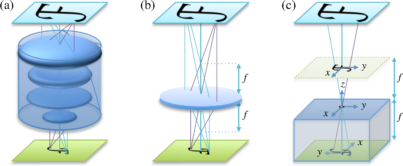

In the pinhole camera, the origin of a coordinate system is fixed at the pinhole and the $z$ -axis is parallel to the optical axis. The plane $z = - f$ , where $f$ is the focal length, is the actual image plane. Note that the image is inverted; therefore, the $x$ and $y$ axes are reverted to describe the image as a magnified version of the object. The inversion of the axes is avoided using the conjugate image plane $z = f$ as shown in Fig. 7(c).

5.1.

Centered Pinhole Camera

A typical representation of a pinhole camera is shown in Fig. 8. The coordinate system $O_{c} x_{c} y_{c} z_{c}$ is known as the camera reference frame. Let

Eq. (68)

p_{c} = {[\begin{matrix} x_{c} & y_{c} & z_{c} \end{matrix}]}^{T}

be the coordinates of a point in the camera reference frame. The point

p_{c}

will be imaged in the plane

z_{c} = f

at the point

Eq. (69)

β = {[\begin{matrix} β_{x} & β_{y} \end{matrix}]}^{T},

where

β

will be referred to as the physical image coordinates. The pinhole projection model relates the vectors

p_{c}

and

β

by

Eq. (70)

[\begin{matrix} β_{x} \\ β_{y} \\ f \end{matrix}] = \frac{f}{z_{c}} [\begin{matrix} x_{c} \\ y_{c} \\ z_{c} \end{matrix}] .

Using homogeneous coordinates for the image point

β

, Eq. (70) can be rewritten as

Eq. (71)

β = H_{f}^{- 1} [p_{c}] = H^{- 1} [Ξ_{f}^{- 1} p_{c}] .

The image formed in the sensor of the camera is sampled as an array of pixels. Then, the physical coordinates

β

will be transformed to the pixel coordinates

Eq. (72)

μ = {[\begin{matrix} u & v \end{matrix}]}^{T},

which depend on the size of the pixel and skew (diagonal distortion) as shown in Fig. 8. The sampling can be described as

Eq. (73)

u = (β_{x} + τ_{x}) / s_{x} + σ β_{y}, v = (β_{y} + τ_{y}) / s_{y},

where

s_{x}

and

s_{y}

(with units of length) are the width and height of the pixel, respectively,

τ = {[τ_{x}, τ_{y}]}^{T}

is known as the principal point and represents the point (from the

u v

-reference frame) where the optical axis crosses the image plane, and

σ

is the skew factor (

σ = 0

for most camera sensors). Equation (73) can be written as

Eq. (74)

[\begin{matrix} u \\ v \\ 1 \end{matrix}] = [\begin{matrix} 1 / s_{x} & σ & τ_{x} / s_{x} \\ 0 & 1 / s_{y} & τ_{y} / s_{y} \\ 0 & 0 & 1 \end{matrix}] [\begin{matrix} β_{x} \\ β_{y} \\ 1 \end{matrix}],

or using a compact notation

Eq. (75)

μ = H^{- 1} [S H [β]] = P_{S} [β],

where

S

is the sampling matrix given as

Eq. (76)

S = [\begin{matrix} 1 / s_{x} & σ & τ_{x} / s_{x} \\ 0 & 1 / s_{y} & τ_{y} / s_{y} \\ 0 & 0 & 1 \end{matrix}] .

Substituting Eq. (71) into Eq. (75), we obtain the image

μ

(in pixel coordinates) of the point

p_{c}

as

Eq. (77)

μ = P_{S} [H^{- 1} [Ξ_{f}^{- 1} p_{c}]] = H^{- 1} [S Ξ_{f}^{- 1} p_{c}] = H^{- 1} [K p_{c}],

where

K = S Ξ_{f}^{- 1}

is known as the matrix of intrinsic camera parameters having the explicit form

Eq. (78)

K = [\begin{matrix} 1 / s_{x} & σ & τ_{x} / f s_{x} \\ 0 & 1 / s_{y} & τ_{y} / f s_{y} \\ 0 & 0 & 1 / f \end{matrix}] .

Since

\det K = {(s_{x} s_{y} f)}^{- 1}

, the matrix

K

is nonsingular for any experimental case.

Fig. 8

The centered pinhole camera and sampling of the image plane.

Given a point $μ$ (in pixel coordinates), the actual coordinates $H_{f} [β]$ of an image point (physical coordinates on the image plane $z = f$ ) can be obtained from Eq. (75) as

Eq. (79)

H_{f} [β] = H_{f} [P_{S^{- 1}} [μ]] = Ξ_{f} H [P_{S^{- 1}} [μ]] = Ξ_{f} S^{- 1} H [μ] / S [S^{- 1} H [μ]] = K^{- 1} H [μ],

where the equality

S [S^{- 1} H [μ]] = 1

was used.

5.2.

Noncentered Pinhole Camera

Let us consider that the pinhole camera is at an arbitrary position and orientation with respect to a world coordinate system $O x y z$ as shown in Fig. 9. The position and orientation of the camera are defined by the vector $t$ and the rotation matrix $R$ , respectively. Let

Eq. (80)

p = {[\begin{matrix} x & y & z \end{matrix}]}^{T}

be a point in the world coordinate system. Then, the point

p

is seen from the camera reference frame as

Eq. (81)

p_{c} = R^{T} (p - t) = L H [p],

where

L

is known as the matrix of extrinsic camera parameters having the explicit form

Eq. (82)

L = [\begin{matrix} R^{T} & - R^{T} t \end{matrix}] .

By substituting Eq. (81) into Eq. (77), the complete imaging process by a noncentered pinhole camera is given as

Eq. (83)

μ = H^{- 1} [K L H [p]] = H^{- 1} [C H [p]],

where

C = K L

is the matrix of the camera.

Fig. 9

The noncentered pinhole camera.

5.3.

Homography Matrix

In general terms, Eq. (83) describes a transformation of points $p$ of the 3-D space to points of the 2-D one. A very useful transformation is obtained when $p$ represents points of a plane in the 3-D space. In this case, Eq. (83) is reduced to a transformation from the 2-D space to itself.

Consider that $p$ represents the points of a plane in the 3-D space; mathematically, see Eq. (53)

Eq. (84)

p = Π H [ρ],

where

ρ = {[ρ_{x}, ρ_{y}]}^{T}

parameterizes the plane,

Π = [q_{1}, q_{2}, s]

is the matrix of the plane,

q_{1}

and

q_{2}

are columns of the rotation matrix

Q = {[q_{1}, q_{2}, q_{3}]}^{T}

, and

s

is a translation vector. Next, the points

p

are transformed to

μ

by Eq. (83) as

Eq. (85)

μ = H^{- 1} [C H [Π H [ρ]]] = H^{- 1} [C [\begin{matrix} Π \\ H {[0_{2}]}^{T} \end{matrix}] H [ρ]] = H^{- 1} [G H [ρ]] = P_{G} [ρ],

where

G

is known as the homography matrix and has the explicit form

Eq. (86)

G = K L [\begin{matrix} Π \\ H [0_{2}] \end{matrix}] = K R^{T} [\begin{matrix} Π & - t H {[0]}^{T} \end{matrix}] = K R^{T} \bar{Π},

where

Eq. (87)

\bar{Π} = [\begin{matrix} Π & - t H {[0]}^{T} \end{matrix}] = [\begin{matrix} q_{1} & q_{2} & s - t \end{matrix}] .

From Eqs. (79) and (85), a point

ρ

is imaged at the point with actual image coordinates

Eq. (88)

H_{f} [β] = K^{- 1} H [μ] = K^{- 1} H [P_{G} [ρ]] = K^{- 1} G H [ρ] / λ = R^{T} \bar{Π} H [ρ] / λ,

where

λ = S [G H [ρ]]

.

The homography matrix is singular when the pinhole is at a point of the reference plane. For any other case, $\det G = q_{3}^{T} (s - t) / (s_{x} s_{y} f)$ and Eq. (85) can be inverted as

Eq. (89)

ρ = P_{G^{- 1}} [μ] .

The homography matrix is very useful for many computer vision tasks. In Appendix A, the direct linear transformation method for homography estimation is described.

6. Perspective Correction for Document Scanning

A camera document scanning application performs several image processing tasks, such as quadrilateral detection, perspective correction, resampling, and image enhancement. In this section, the perspective correction task is addressed to illustrate the application of the proposed approach.

6.1.

Assumptions

In Appendix A, we show that the perspective of a flat object can be easily corrected using the associated homography. For this, at least four correspondences $(μ_{k}, ρ_{k})$ must be provided. However, for practical document scanning, the coordinates $ρ_{k}$ are unknown. Instead, it is assumed that the document to be digitized is rectangular and the orthogonality and parallelism properties of its edges are exploited.

The estimation of the homography is greatly simplified by assuming a centered pinhole camera with known intrinsic parameters; e.g., by a previous camera calibration, see Appendix B. Thus, we only require to estimate the reference plane parameters $Π$ , i.e., the rotation matrix $Q$ and the translation vector $s$ , see Eq. (84).

6.2.

Estimation of the Reference Plane Parameters

Consider a coordinate system in the reference plane with origin at the center of the document to be scanned as shown in Fig. 10(a). The $x$ - and $y$ -axes of this coordinate system are parallel with the upper/lower and left/right sides of the paper, respectively. The corners of the document to be digitized have coordinates given by the vectors

Eq. (90)

ρ_{k}, k = 1, \dots, 4 .

In this configuration, the vectors

ρ_{k}

are symmetric about the

y

-axis; that is

Eq. (91)

ρ_{2} = T ρ_{1}, ρ_{4} = T ρ_{3},

where

Eq. (92)

T = [\begin{matrix} - 1 & 0 \\ 0 & 1 \end{matrix}] .

When the document is imaged by the camera, the original rectangle is transformed to a quadrilateral because of the perspective distortion. The corners of the imaged document have coordinates given by the vectors

Eq. (93)

μ_{k}, k = 1, \dots, 4,

as shown in Fig. 10(b). The vectors

μ_{k}

and

ρ_{k}

are related by Eqs. (85) and (89); however, the vectors

ρ_{k}

and the homography

G

are unavailable. Only the vectors

μ_{k}

are available, which are easily obtained from the image by pointing the vertexes of the imaged document.

Fig. 10

(a) Depict of the rectangular paper to be digitized. (b) The quadrilateral obtained by pinhole imaging of a rectangular paper. (c) The remaining rotation after perspective correction of the quadrilateral shown in (b).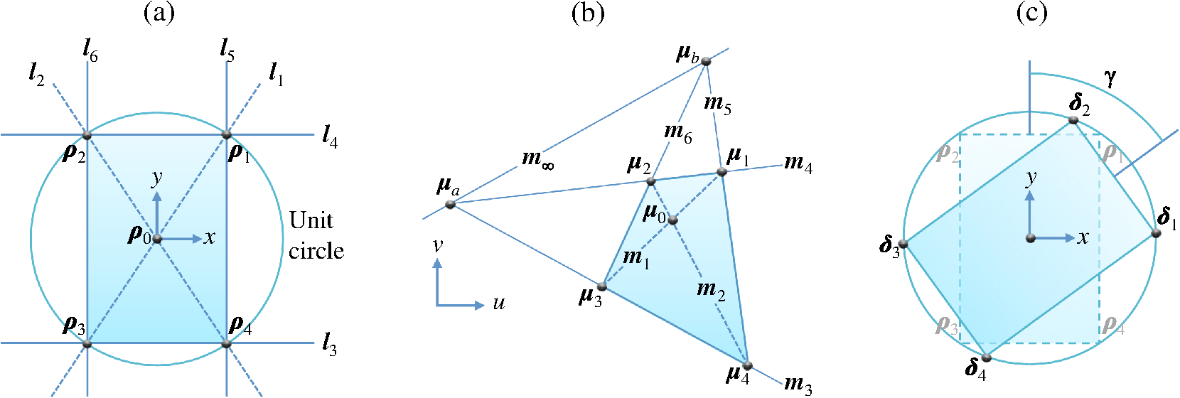

The points $μ_{k}$ are used to compute the following lines, see Fig. 10(b),

Eq. (94)

m_{1} = H [μ_{3}] \times H [μ_{1}], m_{4} = H [μ_{1}] \times H [μ_{2}], m_{2} = H [μ_{2}] \times H [μ_{4}], m_{5} = H [μ_{4}] \times H [μ_{1}], m_{3} = H [μ_{3}] \times H [μ_{4}], m_{6} = H [μ_{2}] \times H [μ_{3}] .

Next, with the lines

m_{k}

, the following three intersection points are computed

Eq. (95)

μ_{0} = H^{- 1} [m_{1} \times m_{2}], μ_{a} = H^{- 1} [m_{3} \times m_{4}], μ_{b} = H^{- 1} [m_{5} \times m_{6}] .

Since the intrinsic camera parameters are assumed to be known, the actual image coordinates of the points

μ_{i}

can be obtained by Eq. (79) as

Eq. (96)

H_{f} [β_{i}] = K^{- 1} H [μ_{i}],

with

i = a, b, 0,1, 2,3, 4

.

6.2.1.

Normal vector

Note that the points $μ_{a}$ and $μ_{b}$ are the projections of the ideal points

Eq. (97)

H [ρ_{a}] = {[\begin{matrix} 1 & 0 & 0 \end{matrix}]}^{T}, H [ρ_{b}] = {[\begin{matrix} 0 & 1 & 0 \end{matrix}]}^{T},

respectively. Thus, the line

m_{\infty}

(in physical coordinates on the image plane

z = f

) is parallel to the normal

q_{3}

, see Eq. (67). That is,

Eq. (98)

n = H_{f} [β_{a}] \times H_{f} [β_{b}] = q_{3} / λ,

for some

λ

. Thus, the normal of the reference plane is obtained as the normalization of the vector

n

, namely

Eq. (99)

q_{3} = n / ‖ n ‖ = \frac{K^{T} [(m_{3} \times m_{4}) \times (m_{5} \times m_{6})]}{‖ K^{T} [(m_{3} \times m_{4}) \times (m_{5} \times m_{6})] ‖} .

6.2.2.

Translation vector

The translation vector $s$ is obtained by taking into account that $P_{G}$ preserves the line–line intersection. Thus, from Eq. (65) we have $μ_{0} = P_{G} [ρ_{0}]$ with $ρ_{0} = 0_{2}$ . Therefore, from Eq. (88) we have

Eq. (100)

H_{f} [β_{0}] = \bar{Π} H [0_{2}] / ξ = s / ξ,

where

ξ

is a scalar to be determined. For this, note that the vectors

Eq. (101)

p_{k} = ζ_{k} H_{f} [β_{k}], k = 1, \dots, 4,

are points of the reference for values

ζ_{k}

and

ξ

such that the equation of the plane

q_{3} (p_{k} - s) = 0

is satisfied. This leads to

Eq. (102)

ζ_{k} = ξ \frac{q_{3}^{T} H_{f} [β_{0}]}{q_{3}^{T} H_{f} [β_{k}]} .

Since the points

ρ_{k}

are on the unit circumference, see Fig. 10(a), then

‖ ρ_{k} ‖ = ‖ p_{k} - s ‖ = 1

, which leads to

Eq. (103)

ξ_{k} = {‖ \frac{q_{3}^{T} H_{f} [β_{0}]}{q_{3}^{T} H_{f} [β_{k}]} H_{f} [β_{k}] - H_{f} [β_{0}] ‖}^{- 1},

where the subindex

k

in

ξ

emphasizes the fact that a different value could be obtained for each

H_{f} [β_{k}]

due to inaccuracies of

μ_{k}

. Therefore, the value

ξ

is computed as

Eq. (104)

ξ = mean {ξ_{1}, ξ_{2}, ξ_{3}, ξ_{4}} .

The result is used in Eq. (100), and the translation of the reference plane is now available.

6.2.3.

Euler angles

The reference plane is fully characterized by six degrees of freedom (DOF), namely position (three coordinates) and orientation (three angles). The vectors $q_{3}$ and $s$ provide five DOFs. Specifically, the vector $s$ provides three DOFs that fix the position while $q_{3}$ provides two DOFs defining the orientation by the azimuth and polar angles given, respectively, by

Eq. (105)

\tan ϕ = q_{23} / q_{13}, \cos θ = q_{33},

where

{[q_{13}, q_{23}, q_{33}]}^{T} = q_{3}

is the third column of the rotation matrix

Q

. The remaining angle

γ

(the angle around the normal

q_{3}

) can be obtained as follows.

From Eqs. (84) and (53), we have

Eq. (106)

p_{k} = Q H_{0} [ρ_{k}] + s,

where the matrix

Q

is defined as the Euler sequence

Eq. (107)

Q = Q_{z} (ϕ) Q_{y} (θ) Q_{z} (γ),

with

Q_{z}

and

Q_{y}

being the rotation matrices around the

z

- and

y

-axes, respectively. Thus, using Eq. (101), the estimated vector

s

, and the angles

θ

and

ϕ

, we compute the (perspective corrected) points

Eq. (108)

δ_{k} = H_{0}^{- 1} [Q_{y}^{T} (θ) Q_{z} {(ϕ)}^{T} (p_{k} - s)] = [\begin{matrix} δ_{x k} \\ δ_{y k} \end{matrix}],

with

k = 1, \dots, 4

, see Fig. 10(c). The vectors

δ_{k}

and

ρ_{k}

are related by

Eq. (109)

ρ_{k} = {\bar{Q}}_{z}^{T} (γ) δ_{k},

where

Eq. (110)

{\bar{Q}}_{z}^{T} (γ) = [\begin{matrix} \cos γ & \sin γ \\ - \sin γ & \cos γ \end{matrix}] .

The vectors

ρ_{k}

are unavailable, but we use their symmetry properties given in Eq. (91) to obtain

Eq. (111)

{\bar{Q}}_{z}^{T} (γ) δ_{2} = T {\bar{Q}}_{z}^{T} (γ) δ_{1}, {\bar{Q}}_{z}^{T} (γ) δ_{4} = T {\bar{Q}}_{z}^{T} (γ) δ_{3} .

The product

{\bar{Q}}_{z}^{T} (γ) δ_{k}

can be written as

Eq. (112)

{\bar{R}}^{T} δ_{k} = B [δ_{k}] Γ,

where

Γ = {[\sin γ, \cos γ]}^{T}

and

Eq. (113)

B [δ_{k}] = [\begin{matrix} δ_{y k} & δ_{x k} \\ - δ_{x k} & δ_{y k} \end{matrix}] .

Thus, Eq. (111) can be rewritten as

Eq. (114)

B Γ = 0_{4},

where

Eq. (115)

B = [\begin{matrix} B [δ_{2}] - T B [δ_{1}] \\ B [δ_{4}] - T B [δ_{3}] \end{matrix}] .

The nontrivial solution of Eq. (114) for

Γ

is obtained as the right-singular vector corresponding to the smallest singular value of

B

. Finally, the angle

γ

is obtained from

Γ

by

Eq. (116)

\tan γ = H^{- 1} [Γ] .

The estimated parameters are used to create the matrix

Π

. Then, the required homography

G

is obtained by Eq. (86) (with

t = 0_{3}

and

R = I

because of the centered pinhole camera configuration). Finally, the perspective distortion of the image is corrected by displaying the intensity of each pixel of the image at the point

ρ

computed by Eq. (89).

6.3.

Illustrative Example

The functionality of the presented algorithm is illustrated by the following example. The camera described in Appendix B and the estimated intrinsic parameters $K$ given in Eq. (156) are used here.

Figure 11(a) shows the image of a rectangular object acquired by the camera. Then, the four corners of the quadrilateral are marked from the image as shown by the yellow circles in Fig. 11(b). The points $μ_{0}$ , $μ_{a}$ , and $μ_{b}$ are indicated by the red circles in Fig. 11(b). It is worth mentioning that $μ_{a}$ , or $μ_{b}$ , or both could be points at infinity. Even in these cases, the presented methodology is valid.

Fig. 11

(a) An input image with a rectangular object in scene. (b) The corners of the rectangle are marked by yellow circles. (c) Corrected image. (d) Zoom of (c) highlighting the region of interest.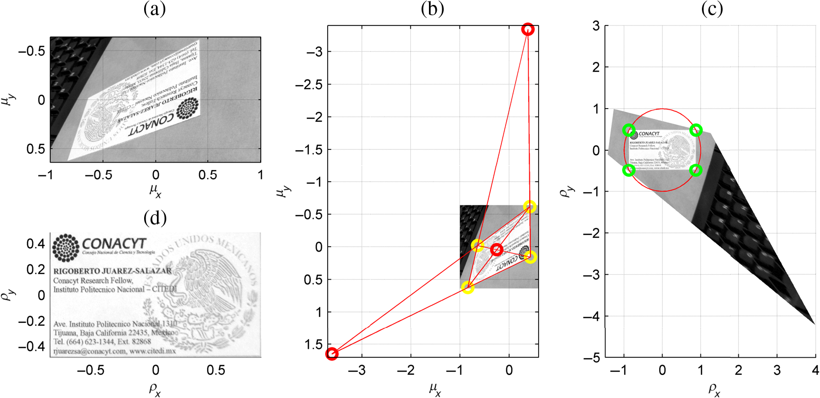

The information estimated with the four corners are

Eq. (117)

s = {[\begin{matrix} - 0.2289 & 0.0561 & 2.9236 \end{matrix}]}^{T}, ϕ = 0.6776, θ = 0.9879, γ = 2.3041 .

With these parameters, the matrix of the reference plane is

Eq. (118)

Π = [\begin{matrix} - 0.7528 & 0.1010 & - 0.2289 \\ 0.3478 & - 0.7779 & 0.0561 \\ 0.5588 & 0.6202 & 2.9236 \end{matrix}] .

Thus, the resulting homography is

Eq. (119)

G = [\begin{matrix} - 2.0219 & 0.2429 & - 0.7272 \\ 0.9237 & - 2.0786 & 0.1298 \\ 0.5588 & 0.6202 & 2.9236 \end{matrix}] .

All points

μ

of the image are transformed to points

ρ

of the reference plane by Eq. (89). Next, the pixels of the image are displayed at the points

ρ

as shown in Fig. 11(c).

With the correction of perspective, the yellow circles in Fig. 11(b) become the green ones in Fig. 11(c). The region of interest is the rectangle with corners marked by green circles in Fig. 11(c). Finally, a zoom of the region of interest is shown in Fig. 11(d).

7. Conclusions

An operator-based approach for homogeneous coordinates was proposed. Several basic geometrical concepts and properties of the operators were investigated. With the proposed approach, the pinhole camera model and a simple camera calibration method were described. The study of this work was motivated by developing a perspective correction method useful for a camera document scanning application. Several experimental results illustrate the analyzed theoretical aspects. The proposed approach could be a good starting point to introduce inexperienced students in the scientific discipline of computer vision.

Appendices

Appendix A:

Estimation of the Homography Matrix

In this appendix, we illustrate the method known as direct linear transformation for homography matrix estimation. This method is very useful for illustration purposes because of its simplicity. However, the highest accuracy and robustness are reached with other advanced methods available in the literature.⁹^,¹³

Let $G$ be the homography matrix defined in Eq. (86). Consider that the matrix $G$ is row partitioned as follows:

Eq. (120)

G = [\begin{matrix} g_{11} & g_{12} & g_{13} \\ g_{21} & g_{22} & g_{23} \\ g_{31} & g_{32} & g_{33} \end{matrix}] = [\begin{matrix} {\bar{g}}_{1}^{T} \\ {\bar{g}}_{2}^{T} \\ {\bar{g}}_{3}^{T} \end{matrix}],

where

Eq. (121)

{\bar{g}}_{1}^{T} = [\begin{matrix} g_{11} & g_{12} & g_{13} \end{matrix}], {\bar{g}}_{2}^{T} = [\begin{matrix} g_{21} & g_{22} & g_{23} \end{matrix}], {\bar{g}}_{3}^{T} = [\begin{matrix} g_{31} & g_{32} & g_{33} \end{matrix}] .

Equation (85), which relates points of the reference and image planes, can be rewritten as

Eq. (122)

μ = [\begin{matrix} u \\ v \end{matrix}] = \frac{1}{{\bar{g}}_{3}^{T} H [ρ]} [\begin{matrix} {\bar{g}}_{1}^{T} H [ρ] \\ {\bar{g}}_{2}^{T} H [ρ] \end{matrix}],

or

Eq. (123)

[\begin{matrix} u {\bar{g}}_{3}^{T} H [ρ] \\ v {\bar{g}}_{3}^{T} H [ρ] \end{matrix}] = [\begin{matrix} {\bar{g}}_{1}^{T} H [ρ] \\ {\bar{g}}_{2}^{T} H [ρ] \end{matrix}] .

Furthermore, Eq. (123) can be written in matrix form as

Eq. (124)

A \bar{g} = 0_{2},

where

Eq. (125)

A = [\begin{matrix} H {[ρ]}^{T} & 0_{3}^{T} & - u H {[ρ]}^{T} \\ 0_{3}^{T} & H {[ρ]}^{T} & - v H {[ρ]}^{T} \end{matrix}], \bar{g} = {[\begin{matrix} {\bar{g}}_{1}^{T} & {\bar{g}}_{2}^{T} & {\bar{g}}_{3}^{T} \end{matrix}]}^{T} .

Equation (124) relates a single point $ρ$ on the reference plane with the corresponding point $μ$ on the image plane. If $n$ pairs $(ρ_{k}, μ_{k})$ , with $k = 1,2, \dots n$ , are available, the $n$ corresponding equations of the form Eq. (124) can be written as

Eq. (126)

A \bar{g} = 0_{2 n},

where

Eq. (127)

A = {[\begin{matrix} A_{1}^{T} & A_{2}^{T} & \dots & A_{n}^{T} \end{matrix}]}^{T}, A_{k} = [\begin{matrix} H {[ρ_{k}]}^{T} & 0_{3}^{T} & - u_{k} H {[ρ_{k}]}^{T} \\ 0_{3}^{T} & H {[ρ_{k}]}^{T} & - v_{k} H {[ρ_{k}]}^{T} \end{matrix}] .

The nontrivial solution $\bar{g}$ of Eq. (126) can be obtained using the constraint $‖ \bar{g} ‖ = 1$ . Thus, by using the singular value decomposition of $A$ , the solution for $\bar{g}$ is the right-singular vector corresponding to the smallest singular value of $A$ , see Appendix C of Ref. 14.

The application of this method is illustrated as follows. Consider the image shown in Fig. 12(a). A letter size paper printed with the Melencolia I by Albrecht Dürer is in the scene. Using the aspect ratio $1 ∶ 1.2941$ of the letter paper, the coordinates of the corners are fixed to

Eq. (128)

ρ_{1} = {[1, 1.2941]}^{T}, ρ_{3} = - ρ_{1}, ρ_{2} = {[- 1, 1.2941]}^{T}, ρ_{4} = - ρ_{2} .

The coordinates of the imaged corners are

Eq. (129)

μ_{1} = {[- 0.2858, 0.5661]}^{T}, μ_{2} = {[0.3826, - 0.0938]}^{T}, μ_{3} = {[- 0.2884, - 0.5403]}^{T}, μ_{4} = {[- 0.8479, - 0.1135]}^{T},

see yellow circles in Fig. 12(a). With these four pairs

(ρ_{k}, μ_{k})

, we obtain the homography

Eq. (130)

G = [\begin{matrix} - 0.2437 & 0.2292 & - 0.2442 \\ 0.2258 & 0.1870 & - 0.0888 \\ - 0.0524 & - 0.0989 & 0.8497 \end{matrix}] .

The homography $G$ fully defines a pinhole imaging process. Thus, it can be inversed to obtain an undistorted view of the reference plane from its perspective distorted image. Specifically, using Eq. (89) all points $μ$ of the image are transformed to points $ρ$ of the reference plane. Then, the pixels of the image are displayed at the points $ρ$ as shown in Fig. 12(b). Note that corners of the paper in the corrected image are at the coordinates specified by Eq. (128).

The least number of point correspondences for two-dimensional homography estimation is four. However, the accuracy of the estimation is improved when more than four point correspondences are provided. For this reason, checkerboard patterns¹⁵ and gratings¹⁶^,¹⁷ are useful target objects. In this appendix, the corner points of the imaged rectangle where obtained manually from the image. However, the corner points can be obtained automatically using checkerboard patterns or gratings along with grid detection¹⁸ or phase demodulation,¹⁹ respectively.

Appendix B:

Camera Parameters from Homographies

The homography matrix involves both intrinsic $K$ and extrinsic $L$ camera parameters as well as the reference plane parameters $Π$ . In this appendix, we show how to obtain the intrinsic and extrinsic camera parameters from several homographies.

B.1.

Intrinsic Camera Parameters

Consider that the reference plane is the $x y$ -plane of the world coordinate system; i.e., $s = 0_{3}$ and

Eq. (131)

\bar{Q} = [\begin{matrix} 1 & 0 \\ 0 & 1 \\ 0 & 0 \end{matrix}] .

In this case, the homography $G$ , defined in Eq. (86), is reduced to

Eq. (132)

G = K [\begin{matrix} {\bar{r}}_{1} & {\bar{r}}_{2} & - R^{T} t \end{matrix}],

where

{\bar{r}}_{1}^{T}

and

{\bar{r}}_{2}^{T}

are the first and second rows of the rotation matrix

R

, respectively. Consider that the matrix

G

is column partitioned as follows:

Eq. (133)

G = [\begin{matrix} g_{11} & g_{12} & g_{13} \\ g_{21} & g_{22} & g_{23} \\ g_{31} & g_{32} & g_{33} \end{matrix}] = [\begin{matrix} g_{1} & g_{2} & g_{3} \end{matrix}],

where

Eq. (134)

g_{1} = [\begin{matrix} g_{11} \\ g_{21} \\ g_{31} \end{matrix}], g_{2} = [\begin{matrix} g_{12} \\ g_{22} \\ g_{32} \end{matrix}], g_{3} = [\begin{matrix} g_{13} \\ g_{23} \\ g_{33} \end{matrix}] .

Thus, Eq. (132) can be written as

Eq. (135)

[\begin{matrix} {\bar{r}}_{1} & {\bar{r}}_{2} & - R^{T} t \end{matrix}] = K^{- 1} [\begin{matrix} g_{1} & g_{2} & g_{3} \end{matrix}] .

Since ${\bar{r}}_{1}$ and ${\bar{r}}_{2}$ are orthonormal vectors ( ${\bar{r}}_{1}$ and ${\bar{r}}_{2}$ are rows of a rotation matrix), we have the following two constraints ${\bar{r}}_{1}^{T} {\bar{r}}_{2} = 0$ and ${‖ {\bar{r}}_{1} ‖}^{2} = {‖ {\bar{r}}_{2} ‖}^{2}$ , which can be written as

Eq. (136)

g_{1}^{T} W g_{2} = 0, g_{1}^{T} W g_{1} = g_{2}^{T} W g_{2},

where the symmetric matrix

W

is defined as

Eq. (137)

W = K^{- T} K^{- 1} = [\begin{matrix} w_{11} & w_{12} & w_{13} \\ w_{12} & w_{22} & w_{23} \\ w_{13} & w_{23} & w_{33} \end{matrix}] .

The bilinear form $g_{i}^{T} W g_{j}$ can be rewritten as

Eq. (138)

g_{i}^{T} W g_{j} = V_{i j} [G] w,

where

Eq. (139)

V_{i j} [G] = {[\begin{matrix} g_{1 i} g_{1 j} \\ g_{2 i} g_{2 j} \\ g_{3 i} g_{3 j} \\ g_{2 i} g_{1 j} + g_{1 i} g_{2 j} \\ g_{3 i} g_{1 j} + g_{1 i} g_{3 j} \\ g_{3 i} g_{2 j} + g_{2 i} g_{3 j} \end{matrix}]}^{T},

and

Eq. (140)

w = {[\begin{matrix} w_{11} & w_{22} & w_{33} & w_{12} & w_{13} & w_{23} \end{matrix}]}^{T} .

Then, the constraints given by Eq. (136) become

Eq. (141)

V [G] w = 0_{2},

where

V [G]

is the following

2 \times 6

matrix:

Eq. (142)

V [G] = [\begin{matrix} V_{12} [G] \\ V_{11} [G] - V_{22} [G] \end{matrix}] .

A nontrivial solution of Eq. (141) for $w$ can be obtained using several homographies $G_{k}$ , $k = 1,2, \dots, m$ . For this, we compute the homographies of different images where the position and orientation of the reference plane (or the camera, or both) are varying (in an unknown manner) while the intrinsic camera parameters remain constant. Thus, we solve the new matrix equation

Eq. (143)

V w = 0_{2 m},

where

Eq. (144)

V = {[\begin{matrix} V {[G_{1}]}^{T} & V {[G_{2}]}^{T} & \dots & V {[G_{m}]}^{T} \end{matrix}]}^{T} .

In general, at least three homographies ( $m = 3$ ) are required. However, two homographies are sufficient assuming zero-skew.

Equation (143) can be solved for $w$ using the singular value decomposition method, see Appendix C of Ref. 14. Since the obtained solution, labeled as $\tilde{w}$ , is unique up to scale, the associated matrix $\tilde{W}$ is related to $W$ by

Eq. (145)

\tilde{W} = λ W = λ K^{- T} K^{- 1},

where

λ \neq 0

is an unknown constant. With the estimated matrix

\tilde{W}

, the unknown scalar

λ

and the entries

k_{i j}

of the intrinsic parameter matrix

Eq. (146)

K = [\begin{matrix} k_{11} & k_{12} & k_{13} \\ 0 & k_{22} & k_{23} \\ 0 & 0 & 1 \end{matrix}],

are given in closed form as

Eq. (147)

λ = (\det \tilde{W}) / d, k_{11} = \sqrt{λ / {\tilde{w}}_{11}}, k_{22} = \sqrt{λ {\tilde{w}}_{11} / d}, k_{12} = - {\tilde{w}}_{12} \sqrt{λ / {\tilde{w}}_{11} d}, k_{13} = ({\tilde{w}}_{12} {\tilde{w}}_{23} - {\tilde{w}}_{22} {\tilde{w}}_{13}) / d, k_{23} = ({\tilde{w}}_{12} {\tilde{w}}_{13} - {\tilde{w}}_{11} {\tilde{w}}_{23}) / d,

where

d = {\tilde{w}}_{11} {\tilde{w}}_{22} - {\tilde{w}}_{12}^{2}

.

It is worth mentioning that the intrinsic camera parameters ( $f$ , $s_{x}$ , $s_{y}$ , $τ_{x}$ , $τ_{y}$ , and $σ$ ) cannot be obtained using only the matrix $K$ . Fortunately, the matrix $K$ is sufficient for many computer vision tasks. For the case where the intrinsic camera parameters are required explicitly, we can assume that the skew and size of the pixel are known (e.g., $s_{x}$ , $s_{y}$ , and $σ$ are consulted in the datasheet of the camera sensor). Thus, the estimation of the remaining intrinsic parameters is a linear problem with the least-squares solution

Eq. (148)

f = s_{x} s_{y} \frac{s_{x} k_{22} + s_{y} k_{11} + s_{x} s_{y} σ k_{12}}{s_{x}^{2} + s_{y}^{2} + s_{x}^{2} s_{y}^{2} σ^{2}},

Eq. (149)

τ_{x} = s_{x} k_{13},

Eq. (150)

τ_{y} = s_{y} k_{23} .

B.2.

Extrinsic Camera Parameters

Once the matrix $K$ is available, the rotation matrix $R$ and the translation vector $t$ can be estimated for each provided homography as follows. First, we compute the estimate ${\tilde{R}}^{T}$ of the matrix $R^{T}$ as

Eq. (151)

{\tilde{R}}^{T} = [\begin{matrix} h_{1} & h_{2} & h_{1} \times h_{2} \end{matrix}],

where using Eq. (135), the vectors

h_{1}

and

h_{2}

are given as

Eq. (152)

h_{1} = K^{- 1} g_{1}, h_{2} = K^{- 1} g_{2} .

Then, the rotation matrix $R$ is obtained from $\tilde{R}$ ensuring the orthogonality condition of rotation matrices. For this, the singular value decomposition $\tilde{R} = U Σ V^{T}$ is obtained and the required rotation matrix is determined as

Eq. (153)

R = U V^{T} .

Finally, the translation vector $t$ is computed as

Eq. (154)

t = - R K^{- 1} g_{3} .

B.3.

Illustrative Example

As an example, we describe a simple experiment to obtain the intrinsic parameters of a camera. A camera with a pixel size of $6 μ m$ (square pixel), resolution of $752 \times 480 pixel$ , and imaging lens with focal length of 6 mm was used. The $3 \times 3$ checkerboard pattern shown in Fig. 13(a) was printed on a letter paper. Then, 15 images of the printed pattern lying on the reference plane were captured from different unknown viewpoints, see Figs. 13(b)–13(i).

We use the coordinates of the corners shown in Fig. 13(a) as the known points $ρ_{k}$ on the reference plane. The corresponding points $μ_{k}$ in the image plane were obtained by marking the corners of the checkerboard pattern in the image. Then, with the pairs $(ρ_{k}, μ_{k})$ , an homography matrix $G_{k}$ was computed for each acquired image. With these homographies, the matrix $V$ defined in Eq. (144) was created. Then, Eq. (143) was solved for $w$ , the resulting matrix $\tilde{W}$ is

Eq. (155)

\tilde{W} = [\begin{matrix} - 0.1389 & 0.0005 & - 0.0058 \\ 0.0005 & - 0.1378 & - 0.0008 \\ - 0.0058 & - 0.0008 & - 0.9806 \end{matrix}] .

From this, the intrinsic parameter matrix $K$ was recovered as

Eq. (156)

K = [\begin{matrix} 2.6563 & - 0.0103 & - 0.0419 \\ 0 & 2.6674 & - 0.0059 \\ 0 & 0 & 1 \end{matrix}] .

For validation purposes, we estimate the focal length using the known information $s_{x} = s_{y} = 6 μ m$ , and $σ = 0$ . The reader should note that the quantities $s_{x}$ and $s_{y}$ are defined in this experiment as

Eq. (157)

s_{x} = s_{y} = \frac{752}{2} 6 \times 10^{- 3} mm

because the points

μ

were obtained in a coordinate system with a unit of length equal to a half of the image width, see Figs. 13(b)–13(i). From the matrix

K

in Eq. (156), the focal length was estimated using Eq. (148). The result is

f = 6.0032 mm

, which is very close to the nominal focal length (6 mm) of the employed camera lens.

Fig. 12

(a) Image of $1168 \times 2080 pixel$ capturing a scene with the Melencolia I printed on a letter size paper. (b) Perspective corrected Image.

Fig. 13

(a) A $3 \times 3$ checkerboard pattern and the coordinates of the corners. (b)–(i) 8 of 15 images of the reference plane acquired by a camera from different unknown viewpoints.

Acknowledgments

This work was supported by CONACyT México through the project Cátedras/880.

References

1.

O. Faugeras, Q.-T. Luong and T. Papadopoulo, The Geometry of Multiple Images: the Laws that Govern the Formation of Multiple Images of a Scene and Some of Their Applications, MIT Press, Cambridge (2004). Google Scholar

2.

O. D. Faugeras and S. Maybank, “Motion from point matches: multiplicity of solutions,” Int. J. Comput. Vision, 4 (3), 225 –246 (1990). http://dx.doi.org/10.1007/BF00054997 IJCVEQ 0920-5691 Google Scholar

3.

Z. Zhang, “A flexible new technique for camera calibration,” IEEE Trans. Pattern Anal. Mach. Intell., 22 1330 –1334 (2000). http://dx.doi.org/10.1109/34.888718 ITPIDJ 0162-8828 Google Scholar

4.

Y. Zhao and Y. Li, “Camera self-calibration from projection silhouettes of an object in double planar mirrors,” J. Opt. Soc. Am. A, 34 696 –707 (2017). http://dx.doi.org/10.1364/JOSAA.34.000696 JOAOD6 0740-3232 Google Scholar

5.

T. Taketomi et al., “Camera pose estimation under dynamic intrinsic parameter change for augmented reality,” Comput. Graphics, 44 11 –19 (2014). http://dx.doi.org/10.1016/j.cag.2014.07.003 Google Scholar

6.

H. H. Ip and Y. Chen, “Planar rectification by solving the intersection of two circles under 2D homography,” Pattern Recognit., 38 (7), 1117 –1120 (2005). http://dx.doi.org/10.1016/j.patcog.2004.12.004 PTNRA8 0031-3203 Google Scholar

7.

B. Cyganek and J. P. Siebert, An Introduction to 3D Computer Vision Techniques and Algorithms, John Wiley & Sons Ltd., Chichester, West Sussex (2009). Google Scholar

8.

O. Faugeras, Three-Dimensional Computer Vision: a Geometric Viewpoint, MIT Press, Cambridge (1993). Google Scholar

9.

R. Hartley and A. Zisserman, Multiple View Geometry in Computer Vision, Cambridge University Press, Cambridge (2003). Google Scholar

10.

J. L. Mundy and A. Zisserman, Appendix—Projective Geometry for Machine Vision, 463 –519 MIT Press, Cambridge (1992). Google Scholar

11.

W. Burger, “Zhang’s camera calibration algorithm: in-depth tutorial and implementation,” Hagenberg, Austria (2016). Google Scholar

12.

F. Devernay and O. Faugeras, “Straight lines have to be straight,” Mach. Vision Appl., 13 (1), 14 –24 (2001). http://dx.doi.org/10.1007/PL00013269 MVAPEO 0932-8092 Google Scholar

13.

H. Zeng, X. Deng and Z. Hu, “A new normalized method on line-based homography estimation,” Pattern Recognit. Lett., 29 (9), 1236 –1244 (2008). http://dx.doi.org/10.1016/j.patrec.2008.01.031 PRLEDG 0167-8655 Google Scholar

14.

Z. Zhang, “A flexible new technique for camera calibration,” (1998). Google Scholar

15.

L. Kr, “Accurate chequerboard corner localisation for camera calibration,” Pattern Recognit. Lett., 32 (10), 1428 –1435 (2011). http://dx.doi.org/10.1016/j.patrec.2011.04.002 PRLEDG 0167-8655 Google Scholar

16.

R. Juarez-Salazar et al., “Camera calibration by multiplexed phase encoding of coordinate information,” Appl. Opt., 54 4895 –4906 (2015). http://dx.doi.org/10.1364/AO.54.004895 APOPAI 0003-6935 Google Scholar

17.

R. Juarez-Salazar, L. N. Gaxiola and V. H. Diaz-Ramirez, “Single-shot camera position estimation by crossed grating imaging,” Opt. Commun., 382 585 –594 (2017). http://dx.doi.org/10.1016/j.optcom.2016.08.041 OPCOB8 0030-4018 Google Scholar

18.

A. Herout, M. Dubská and J. Havel, Vanishing Points, Parallel Lines, Grids, 41 –54 Springer, London (2013). Google Scholar

19.

R. Juarez-Salazar, F. Guerrero-Sanchez and C. Robledo-Sanchez, “Theory and algorithms of an efficient fringe analysis technology for automatic measurement applications,” Appl. Opt., 54 5364 –5374 (2015). http://dx.doi.org/10.1364/AO.54.005364 APOPAI 0003-6935 Google Scholar

Biographies for the authors are not available.

Citation Download Citation

Rigoberto Juarez-Salazar and Victor H. Díaz-Ramírez "Operator-based homogeneous coordinates: application in camera document scanning," Optical Engineering 56(7), 070801 (27 July 2017). https://doi.org/10.1117/1.OE.56.7.070801

Received: 11 May 2017; Accepted: 7 July 2017; Published: 27 July 2017

Access the abstract

JOURNAL ARTICLE
16 PAGES

DOWNLOAD PAPER SAVE TO MY LIBRARY

GET CITATION

CITATIONS

Cited by 25 scholarly publications.

Explore citations on Lens.org

RIGHTS & PERMISSIONS

Get copyright permission Get copyright permission on Copyright Marketplace

Subscribe to Digital Library

Receive Erratum Email Alert

1.

Introduction

2.

Definition of Operators

2.1.

Operators H and S

Eq. (1)

Eq. (2)

Eq. (3)

Eq. (4)

Eq. (5)

Eq. (6)

Eq. (7)

Eq. (8)

Eq. (9)

Eq. (10)

Eq. (11)

Eq. (12)

Eq. (13)

2.2.

Projection Operator P

Eq. (14)

Eq. (15)

Eq. (16)

Eq. (17)

Eq. (18)

Table 1

3.

One-Dimensional Space

Fig. 1

Eq. (19)

Eq. (20)

3.1.

Ideal Point

Eq. (21)

Eq. (22)

Eq. (23)

Fig. 2

Eq. (24)

3.2.

One-Dimensional Projection

Eq. (25)

Eq. (26)

Eq. (27)

Fig. 3

4.

Two-Dimensional Space

4.1.

Points and Lines in the Plane

Eq. (28)

Eq. (29)

Eq. (30)

Eq. (31)

Eq. (32)

Fig. 4

Eq. (33)

Eq. (34)

Eq. (35)

4.2.

Parallel Lines

Eq. (36)

Eq. (37)

Eq. (38)

Eq. (39)

Eq. (40)

Eq. (41)

Eq. (42)

4.3.

Ideal Points and the Line at Infinity

Eq. (43)

Eq. (44)

Eq. (45)

Eq. (46)

Eq. (47)

Eq. (48)

Eq. (49)

Eq. (50)

Eq. (51)

Eq. (52)

Fig. 5

Operators $H$ and $S$

Projection Operator $P$