1.

Introduction

Recently, a noncontact light detector utilizing a purposely designed microlens array (MLA-D) has been developed.¹ The detector consisted of a MLA, a septum mask, and a photon sensor [cf. Fig. 1(a)]. In contrast to conventional lens-based imaging systems, an MLA-D possesses a thin construction size ($<10\mathrm{mm}$ including cooling). Since its imaging performance is optimal for objects positioned close to its optics, a single or a multitude of MLA-Ds can be arranged circumferentially in close proximity to the imaged object, hence allowing for confined system assembly. Furthermore, the whole optical imaging system can potentially be encircled by another imaging system such as positron emission tomography or magnetic resonance imaging (MRI), in which MLA-Ds are compatible or nearly “invisible.”²

Fig. 1

Cross-sectional view of the microlens-based optical detector (MLA-D) containing a microlens array (MLA), a septum mask, and a photon sensor (a). Experimental data of adjacent elemental images (EIs) using an assembled MLA-D, as listed in setup 1 (Table 1). Each EI contains $1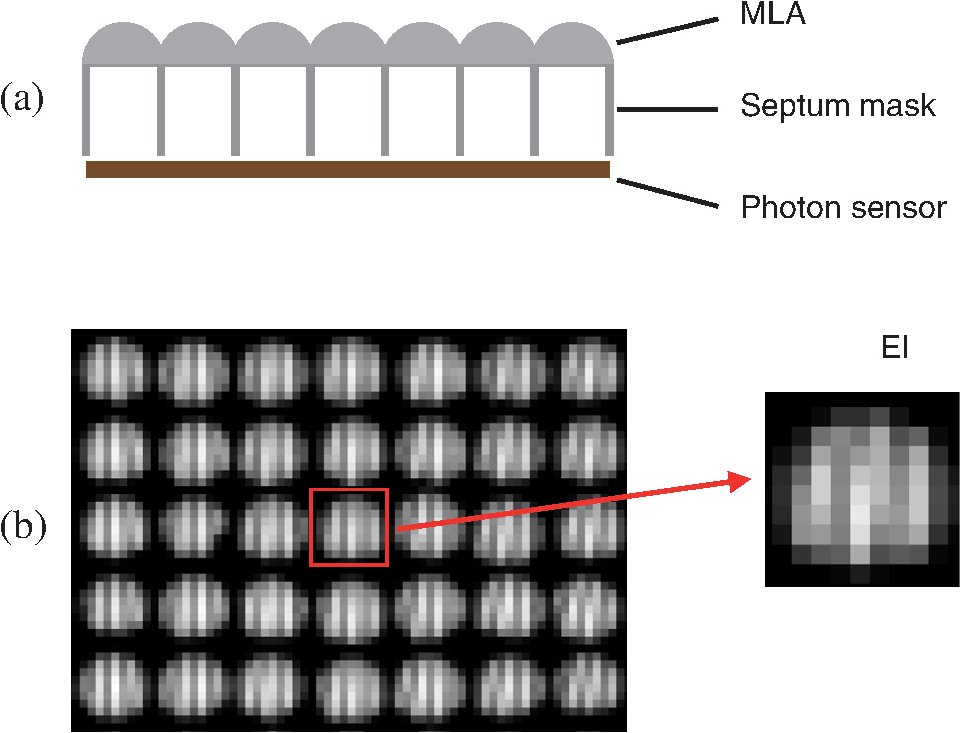0\times 10\text{pixels}$ (b).

An MLA-D does not form an immediate observer image. Corresponding to each microlens, a local lattice of sensor pixels forms a so-called elemental image (EI), as shown in Fig. 1(b). Therefore, an image needs to be calculated by inverse mapping³ or an iterative algorithm, as depicted in Ref. 4. For noncontact optical in vivo imaging, the procedure for localizing emitted photons within the imaged object—with the purpose to further solve the inverse problem involved in image reconstruction^5,6—is crucially affected by the exact knowledge of the three-dimensional (3-D) surface of the imaged object. As of today, surface information is mainly derived from secondary data as provided by (1) imaging the object with another modality such as x-ray computed tomography (CT)⁵ or MRI⁷ or (2) conducting a structured light 3-D scanning procedure.⁸ Alternatively, direct optical methods such as back-projection-based (silhouette or visual hull) based approaches have also been proposed.^9–11 While the first class of methods requires additional hardware and scanning steps, the second class is generally considered less accurate, as concave areas cannot always be resolved.

As both classes of approaches operate independently from the light camera being used, they have been proposed in the literature (a survey is given in Ref. 12) as either conventional or multilens-based camera approaches such as the MLA-D employed here.^13,14 For the latter systems though, it has been shown recently that 3-D imaging, including surface reconstruction, can be achieved by so-called integral imaging techniques.^15,16

Using MLAs to record and recover light fields has become a recent research highlight in the fields of optics and computer vision.^17–19 Shape reconstruction or depth retrieval using MLAs can be performed from a single projection by finding corresponding points among neighboring EIs or adjacent focal point images.^15,20 Due to the limited number of microlenses and/or light trajectories, the reconstructed surface possesses a rather low-depth resolution and is insufficient for the downstream task of image reconstruction from optical data (tomography).

Considering that the MLA-D is either part of a multidetector imaging setup or is positioned or rotated around the imaged object, the aforementioned problem could be improved upon by combining multiple projections from multiview data (at unchanged illumination condition), which has been extensively studied in computer vision.^21–23 However, the direct application of these algorithms in the MLA-D system is difficult for two main reasons. First, global illumination either by environmental light or by fixed distributed light sources is difficult to achieve due to the enclosed design.¹ Second, the EIs of the MLA-Ds possess a comparatively low resolution so the visibility computation is difficult to perform.

Therefore, an integrated instrumentation setup for in vivo small animal (mice) imaging is presented by means of a simulation study employing MLA-Ds of various sizes as well as by a new light source setup for object illumination. Furthermore, a dedicated surface reconstruction algorithm is presented for this setup, which is based on a newly defined photo-consistency measure (the concept of photo-consistency measure can be referred in Ref. 22) and volumetric graph cuts. It is particularly tailored to the comparatively large number of EIs in our design, albeit each EI possesses a rather low-spatial resolution.

2.

Methods

2.1.

MLA-D

As depicted in Fig. 2, the binary sensor data of an MLA-D represents a two-dimensional (2-D) matrix $\mathbf{B}=[b_{m,n}](m=1,\cdots M;n=1,\cdots N)$ with square pixel size $p$, where $M$ and $N$ are the number of pixels in $x$ and $y$ directions on the photosensor plane, respectively. The arrangement of sensor-aligned $G\times H$ microlenses with lens pitch $d_l$ is represented by $\mathbf{L}=[l_{g,h}](g=1,\cdots G;h=1,\cdots H)$. An elemental image $\mathbf{E}$ is formed with local pixels corresponding to microlens $l_{g,h}$, represented as $\mathbf{E}=[e_{u,v}](u=1,\cdots U;v=1,\cdots V)$, where $U$ and $V$ are the numbers of pixels in 2-D for each EI in $x$ and $y$ directions, respectively.

Fig. 2

Illustration of MLA-D notation.

Currently, two types of MLA-D setups have been proposed,^1,14 for which the parameters are summarized in Table 1, respectively. The first design has been assembled and is being used in practice, whereas the second is still under construction.

Table 1

Microlens array-based light detector (MLA-D) specification for the simulation setups.

Parameter	Setup 1	Setup 2
Focal length, $f$ (mm)	2.2	2.4
Lens pitch, $d_l$ (μm)	480	520
Half-cone angle, $\theta$ (deg)	6.2	6.2
Pixel size, $p$ (μm)	48	6.5
Lens grid, $G\times H$	$70\times 60$	$64\times 54$
Sensor resolution, $M\times N$	$700\times 600$	$5120\times 4320$
Elemental image (EI) resolution, $U\times V$	$10\times 10$	$80\times 80$
Detector size (${\mathrm{mm}}^2$)	$33\times 28$	$33\times 28$

2.2.

System Simulation

The simulation is performed within the physically based rendering (PBRT) framework, which includes interfaces for detector, lighting, and scenario (imaged object) descriptions.²⁴ The configuration of the MLA-Ds is defined by the parameters in Table 1. As a result of the previously mentioned illumination source confinement, a local illumination setup as illustrated in Fig. 3 is selected. As can be seen, adjacent MLA-Ds share the same illumination. The whole assembly is also rotatable around the long axis of the imaged object to acquire the data at $A$ angular views. At each projectional view, two sensor data, ${\mathbf{B}}_a^1$ and ${\mathbf{B}}_a^2$ $(a=1,\dots ,A)$, are obtained from the detectors.

Fig. 3

Geometry of the proposed system design and notations. This design ensures a local illumination condition, because two MLA-Ds share the illumination by a pair of fixed diffuse line sources. When the system rotates, both MLA-Ds and light sources rotate at the same offset.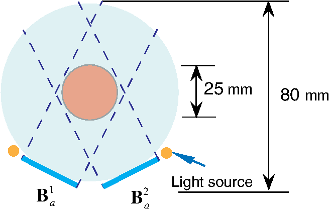

In order to define a realistic phantom representing an imaged object, a triangulated mesh extracted from a nude mouse CT dataset²⁵ is adopted as input for the simulation, as shown in Fig. 4. The actual (identical) fields of view (FOVs) of the simulated MLA-Ds are marked by the red box. Once the surface data have been derived, its reflectance is set to be ideally diffusive (Lambertian surface).^26,27 Considering the size of normal mice (approximately 25 mm in diameter) as well as the depth of field for the individual microlenses, the radius of rotation is set to be 40 mm. The oblique angle between the two detectors is set to be 40 deg in order to maintain the condition that any point on the surface of the imaged object is being seen on either detector (photo-consistency). Further details about the simulation can be found in Ref. 14. The simulation is carried out by employing a high-performance computer cluster with 128 CPU cores (Intel E5450, 3.0 GHz, 16 GB memory for each core) for parallel implementation of different microlens units.

Fig. 4

Exemplary projection image of a real mouse CT data acquisition. A triangulated mesh is derived from the CT volume and acts as the phantom for the simulation. The box marked in red refers to the desired region of interest, as imaged by the MLA-Ds.

2.3.

Surface Reconstruction

Centrally important to the surface reconstruction procedure, a photo-consistency measure is proposed by comparing the formed EIs following the system shown in Fig. 3. By calculating and super-positioning all photo-consistency measures, a photo-consistency volume of the imaged object is obtained. The problem of surface reconstruction is applied onto the formed volume, concretely to decide whether any voxel belongs to the imaged object, also known as labeling problem.²⁸ The labeling problem can be expressed as an energy minimization form and is further solved by the graph cuts-based method.²⁹

2.3.1.

Photo-consistency measure

To solve the problem of surface reconstruction from multiview stereo in computer vision, a number of approaches have been proposed for evaluating the visual compatibility of a reconstruction with a collection of input images.³⁰ Most of these measures (often entitled photo-consistency measures) operate by comparing pixels in one image to pixels in other images to see how well they correlate.²¹ To define a suitable measure for the surface reconstruction employing the MLA-D configuration, notations are first introduced.

In the process of image formation, any point $\mathbf{P}(x,y,z)$ on the surface of the imaged object, which is within the FOV of either MLA-D, can potentially be detected by a number of microlenses. A ray originating from $\mathbf{P}(x,y,z)$ that forms a trajectory forward an EI is called a valid ray. A set of EIs containing all valid rays $\widehat{\mathbf{T}}$ of a given $\mathbf{P}(x,y,z)$ is referred to as $\widehat{\mathbf{E}}$, as shown in Fig. 5. The intensities as collected by the sensor of the formed trajectories $\widehat{\mathbf{T}}$ tend to be similar since the corresponding sensor pixels in $\widehat{\mathbf{E}}$ measure the same point $\mathbf{P}$ in space, only from slightly different angles. Instead of comparing the absolute differences among the collected trajectories directly, a more robust method is to compare the similarities between two pixel windows since area matching (pixel window) compares regularly sized regions of pixel values in two images and, hence, is well suited for a texture scene.³¹ For example, two arbitrary trajectories ${\mathbf{T}}_r$ and ${\mathbf{T}}_p$ from $\widehat{\mathbf{T}}$ can be extended to form corresponding pixel windows ${\mathbf{W}}_p$ and ${\mathbf{W}}_r$, respectively (for setup 1, a $3\times 3\text{pixel}$ window is used, while for setup 2, a $7\times 7\text{pixel}$ window is used). The collection of pixel windows is represented as $\widehat{\mathbf{W}}$. Following common strategies assessing similarities between data formed by two pixel windows, the normalized cross-correlation (NCC) is employed in this article as a similarity measure. It is defined as³¹

Eq. (1)

$$\mathrm{NCC}({\mathbf{W}}_p,{\mathbf{W}}_r)=\frac{\sum _{i,j}({\mathbf{W}}_p^{i,j}-{\overline{\mathbf{W}}}_p)({\mathbf{W}}_r^{i,j}-{\overline{\mathbf{W}}}_r)}{\sqrt{\sum _{i,j}{({\mathbf{W}}_p^{i,j}-{\overline{\mathbf{W}}}_p)}^2}\sqrt{\sum _{i,j}{({\mathbf{W}}_r^{i,j}-{\overline{\mathbf{W}}}_r)}^2}},$$

where ${\overline{\mathbf{W}}}_p$ and ${\overline{\mathbf{W}}}_r$ represent the average value of two corresponding pixel windows, respectively. This function yields return values between $-1$ and 1. A perfect match would reach the maximum of 1. In our context, a high correlation is defined ($\mathrm{NCC}>0.7$), which is used in the following part. Employing the NCC function as described decreases the effect of noise in the data due to, among others, the inhomogeneous responses of sensor pixels.

Fig. 5

Illustration of image formation by a single point. Any point $\mathbf{P}$ would form a set of trajectories ($\widehat{\mathbf{T}}$) corresponding to multiple EIs ($\widehat{\mathbf{E}}$). In order to estimate similarities among trajectories, the correlation among pixel windows ($\widehat{\mathbf{W}}$) is derived.

In surface reconstruction procedure, a volume model is adopted to represent the surface for its simplicity and uniformity.²¹ A reasonable simplification can be made, though. Any voxel ${\mathbf{V}}_{i,j,k}$ (the concept “voxel” here refers to a point in a spatial grid) can form trajectories onto the photon sensor plane assuming that there would be no self-occlusion caused by other voxels.²² Using the proposed design as illustrated in Fig. 3, a voxel ${\mathbf{V}}_{i,j,k}$ can be seen through $Q^1$ and $Q^2$ microlenses in the two MLA-Ds simultaneously. Hence, $\widehat{\mathbf{E}}$, $\widehat{\mathbf{T}}$, as well as $\widehat{\mathbf{W}}$ are formed by two subsets: ${\widehat{\mathbf{E}}}^1$ and ${\widehat{\mathbf{E}}}^2$; ${\widehat{\mathbf{T}}}^1$ and ${\widehat{\mathbf{T}}}^2$; and ${\widehat{\mathbf{W}}}^1$ and ${\widehat{\mathbf{W}}}^2$, as shown in Fig. 6.

Fig. 6

An arbitrary point ${\mathbf{V}}_{i,j,k}$ forms pixel windows on MLA-Ds represented as $\widehat{\mathbf{W}}$ (${\widehat{\mathbf{W}}}_1$ and ${\widehat{\mathbf{W}}}_2$ on two detectors, respectively). One pixel window ${\mathbf{W}}_r$ is chosen as reference window (correspondingly, the EI formed is represented as ${\mathbf{E}}_r$). Some pixel windows in $\widehat{\mathbf{W}}$ possess high correlations with ${\mathbf{W}}_r$, while others do not (a). Supposing that there exists an optic ray (dashed line marked in red) between ${\mathbf{V}}_{i,j,k}$ and the optical center $\mathbf{C}$ of the corresponding microlens forming ${\mathbf{E}}_r$, any point $R(d)$ on the optic ray would form the same pixel window ${\mathbf{W}}_r$ within ${\mathbf{E}}_r$. When $R(d)$ is on the surface, the formed pixel windows in $\widehat{\mathbf{W}}$ have high correlations with ${\mathbf{W}}_r$, as seen in (b).

Because of the specific design and configuration of MLA-Ds, the problem of defining a photo-consistency measure is extended from pair comparison between pixel windows, as seen in Eq. (1), to formalize a new measure over two subsets of EIs (${\widehat{\mathbf{E}}}^1$ and ${\widehat{\mathbf{E}}}^2$) and the corresponding pixel windows (${\widehat{\mathbf{W}}}^1$ and ${\widehat{\mathbf{W}}}^2$). A simple method is to choose one reference pixel window ${\mathbf{W}}_r$ within the elemental image ${\mathbf{E}}_r$ from $\widehat{\mathbf{W}}$ and to compare it with the other formed pixel windows from the same subset $\widehat{\mathbf{W}}$, one by one. For an arbitrary ${\mathbf{V}}_{i,j,k}$, it might occur that some of the pixel windows possess a high degree of correlation with ${\mathbf{W}}_r$, while some other pixel windows possess a low degree of correlation, as seen in Fig. 6(a). Although the direct average of all NCC values could be applied, the resolvability among adjacent voxels might be hampered.²²

Therefore, an alternative method is used. The assumption is made that there exists an optic ray between ${\mathbf{V}}_{i,j,k}$ and the optical center $\mathbf{C}$ of a chosen microlens, as depicted in Fig. 6(b). Correspondingly, the formed pixel window of this microlens is chosen as reference pixel window ${\mathbf{W}}_r$. As depicted in Fig. 6(b), an arbitrary point $\mathbf{R}(d)$ on the supposed optic ray defined by ${\mathbf{V}}_{i,j,k}$ and $\mathbf{C}$ could be expressed according to

Eq. (2)

$$\mathbf{R}(d)={\mathbf{V}}_{i,j,k}+d(\mathbf{C}-{\mathbf{V}}_{i,j,k}),$$

where $d$ is a variable to control the position of $\mathbf{R}(d)$. $\mathbf{R}(d)$ would form the same pixel window ${\mathbf{W}}_r$ within the corresponding ${\mathbf{E}}_r$ as $d$ changes, as shown in Fig. 6(b).

However, in any other EI, e.g., a fixed ${\mathbf{E}}_f$ from $\widehat{\mathbf{E}}$ that can detect ${\mathbf{V}}_{i,j,k}$, $\mathbf{R}(d)$ would form different pixel windows as compared with the pixel window formed by ${\mathbf{V}}_{i,j,k}$ within ${\mathbf{E}}_f$. The newly formed pixel window series by $\mathbf{R}(d)$ is represented as ${\widehat{\mathbf{W}}}_f$ as $d$ changes. When comparing ${\mathbf{W}}_r$ with the formed set ${\widehat{\mathbf{W}}}_f$, a maximum NCC value can be found with respect to $d$. If ${\mathbf{V}}_{i,j,k}$ is on the surface (or very close to the surface of the object), the degree of correlation becomes a maximum at $d=0$, as seen in Fig. 7. Contrarily, if ${\mathbf{V}}_{i,j,k}$ is not on the surface, the degree of correlation is lower at $d=0$ or becomes a maximum at $d\ne 0$, as shown in Fig. 6(b). In other words, the maximum value of NCC at $d=0$ can be used as a strong indicator for determining whether ${\mathbf{V}}_{i,j,k}$ is a point on the surface or not.

Fig. 7

When voxel ${\mathbf{V}}_{i,j,k}$ is on the surface of the imaged object, the chosen reference window ${\mathbf{W}}_r$ possesses a high degree of correlation with other pixel windows at $d=0$ (a). When $d$ changes, some pixel windows in $\widehat{\mathbf{W}}$ possess high correlations with ${\mathbf{W}}_r$, while others do not (b).

Having discussed the case of mapping ${\mathbf{V}}_{i,j,k}$ with one microlens, we extend this principle to combine ${\mathbf{V}}_{i,j,k}$ with multiple microlenses. Supposing $N_a$ microlenses are chosen in the $a$-th projection, the number of occurrences, $M_a$, in which a maximum NCC value is derived at $d=0$, would be counted. The ratio $M_a/N_a$ can be used to describe the degree whether ${\mathbf{V}}_{i,j,k}$ is on the surface concerning the normalization effect.

In order to reduce the computational complexity, the following strategies are employed. First, ${\mathbf{W}}_r$ and ${\widehat{\mathbf{W}}}_f$ are chosen from two different detectors. Reasoning is due to the fact that the MLA-Ds configuration is symmetric, as seen in Fig. 3. If there is a case that $N_a$ microlenses are chosen from the first MLA-D detector while $M_a$ occurrences with maximum NCC are obtained on the second MLA-D, equivalently, then it could occur that $N_a^{\prime }$ microlenses are chosen from the second MLA-D detector while $M_a^{\prime }$ occurrences are obtained on the first MLA-D. Second, only EIs within limited $s$ rows (${\widehat{\mathbf{E}}}_1$) are chosen for ${\mathbf{W}}_r$, and $t$ rows of EIs (${\widehat{\mathbf{E}}}_2$) are chosen for ${\widehat{\mathbf{W}}}_f$ ($s$ and $t$ are set as 3, in this article). The photo-consistency measure $\phi ({\mathbf{V}}_{i,j,k})$ is defined as

Eq. (3)

$$\phi ({\mathbf{V}}_{i,j,k})=\exp [-\mu \frac{\sum \frac{M_a({\mathbf{V}}_{\mathbf{i},\mathbf{j},\mathbf{k}})}{N_a({\mathbf{V}}_{\mathbf{i},\mathbf{j},\mathbf{k}})}+\frac{M_a^{\prime }({\mathbf{V}}_{i,j,k})}{N_a^{\prime }({\mathbf{V}}_{i,j,k})}}{2V_A}],$$

in which $\mu$ is a rate-of-decay parameter (set to be 0.5, in this article), and $V_A$ is the number of effective projectional views ($M_a/N_a>0.001$ and $M_a^{\prime }/N_a^{\prime }>0.001$). The details about the implementation could be found in Algorithm 1.

Algorithm 1

Photo-consistency measure calculation.

Input:

${\mathbf{V}}_{i,j,k}$, ${\widehat{\mathbf{B}}}_{fov}=[{\mathbf{B}}_a^1,{\mathbf{B}}_a^2](a=1\cdots A)$

Begin:

Initialize $V_A=0$

for each ${\mathbf{B}}_a^1$, ${\mathbf{B}}_a^2$ in ${\widehat{\mathbf{B}}}_{\mathrm{fov}}$

Choose ${\widehat{\mathbf{E}}}_1$ within $s$ rows of EI’s from first detector and corresponding lens center information

Choose ${\widehat{\mathbf{E}}}_2$ within $t$ rows of EI’s from second detector

BeginPixel windows-comparison:

${\mathbf{V}}_{i,j,k}$ is visible through $N_a({\mathbf{V}}_{i,j,k})$ microlenses in ${\widehat{\mathbf{E}}}_1$

Reference pixel windows set: ${\widehat{\mathbf{W}}}_r=[{\mathbf{W}}_r^l](l=1\cdots N_a)$

Optical center of $N_a$ microlenses: $\widehat{\mathbf{C}}=[{\mathbf{C}}_l](l=1\cdots N_a)$

${\mathbf{V}}_{i,j,k}$ is visible through $F({\mathbf{V}}_{i,j,k})$ microlenses in ${\widehat{\mathbf{E}}}_2$

${\widehat{\mathbf{E}}}_2^F=[{\mathbf{E}}_f](f=1\cdots F)$

Initialize $M_a({\mathbf{V}}_{i,j,k})=0$

for each ${\mathbf{W}}_r^l$ in ${\widehat{\mathbf{W}}}_r$

for each ${\mathbf{E}}_f$ in ${\widehat{\mathbf{E}}}_2^F$

for each $d$

$\mathbf{R}(d)={\mathbf{V}}_{i,j,k}+d({\mathbf{C}}_l-{\mathbf{V}}_{i,j,k})$

Calculate formed pixel window ${\mathbf{W}}_f$ within ${\mathbf{E}}_f$ by $\mathbf{R}(d)$

Calculate NCC value between ${\mathbf{W}}_r^l$ and ${\mathbf{W}}_f$

end loop for $d$

if NCC between ${\mathbf{W}}_r^l$ and ${\mathbf{W}}_f$ reaches maximum at $d=0$

$M_a({\mathbf{V}}_{i,j,k})++$

end loop for ${\mathbf{E}}_l$

end loop for ${\mathbf{W}}_r$

end Pixel window-comparison:

Choose ${\widehat{\mathbf{E}}}_1$ within $s$ rows of EI’s from second detector and corresponding lens center information

Choose ${\widehat{\mathbf{E}}}_2$ within $t$ rows of EI’s from first detector

Do Pixel window-comparison again to obtain $N_a^{\prime }$ and $M_a^{\prime }$

if$M_a/N_a>0.001$ and $M_a^{\prime }/N_a^{\prime }>0.001$

$V_A++$

end loop for ${\mathbf{B}}_a^1$, ${\mathbf{B}}_a^2$

Photo-consistency: $\phi ({\mathbf{V}}_{i,j,k})=\exp (-\mu \frac{\sum \frac{M_a({\mathbf{V}}_{\mathbf{i},\mathbf{j},\mathbf{k}})}{N_a({\mathbf{V}}_{\mathbf{i},\mathbf{j},\mathbf{k}})}+\frac{M_a^{\prime }({\mathbf{V}}_{i,j,k})}{N_a^{\prime }({\mathbf{V}}_{i,j,k})}}{2V_A})$

2.3.2.

Volumetric surface reconstruction based on graph cuts

By calculating the proposed photo-consistency for each voxel employing Eq. (3), a volume of the imaged object is derived. The surface reconstruction task in this context is to assign a label to each voxel of the image object, i.e., a voxel either belongs to the background or to the imaged object. In accordance with labeling a voxel, an energy cost is paid. The objective is to find a discrete labeling of voxels with minimum systematic total energy, known as labeling problem.²⁸ In our context of a binary labeling problem (only two labels for the background and the imaged object), two energy parts are included. One part of cost concerns the label itself (data cost), i.e., the volume of imaged object in this context. This part of total cost can be seen as a volume integration of the imaged object. The other part of cost concerns the regularity of labels among neighboring voxels (regularity cost). When two neighboring voxels have the same label, the regularity cost is zero, whereas two neighboring voxels with the different labels yield nonzero regularity cost values. The regularity cost in this case is set to be the value of the photo-consistency measure calculated by Eq. (3). Because regularity cost is valid across the boundary between the imaged object and its background, the total cost of this part can be seen as a surface integration of the photo-consistency measure. The surface reconstruction problem is transformed to extract an optimal surface $S_{\mathrm{opt}}$, over which the surface integral of the photo-consistency measure $\phi (\mathbf{V})$ is minimized as well as the volume $V(S)$ enclosed by $S_{\mathrm{opt}}$ is maximized. This can be expressed as minimization of the following equation:²²

Eq. (4)

$$E(S)={\iint }_S\phi (\mathbf{V})\mathrm{d}A-\lambda \int \int {\int }_{V(S)}\mathrm{d}V,$$

in which $\lambda$ is a parameter to control the weight of volume integration ($\lambda$ is set to be within 0.05 and 0.25, in this article). In this context, the first term in Eq. (4) is comprehended to be a collapsing force, whereas the second term of volume integration is comprehended to be an expansion force.

The optimization problem in Eq. (4) is solved by the graph-cuts-based method using the implementation by Boykov et al. with expansion moves and swap moves.²⁹ Each voxel is treated as a node in a graph. Given the initial estimation of the imaged object as shown in Fig. 8, i.e., voxels inside of surface $S_{\mathrm{in}}$, the total cost would decrease as the nodes expand. This expansion would stop at the surface of the imaged object, i.e., the balance between the collapsing and ballooning forces (provided that any voxel on the surface possesses a much lower photo-consistency measure, and a good choice of $\lambda$ as indicated above). The convergence and efficiency of this approach has been validated in previous studies.³²

Fig. 8

Illustration of how the optimal surface is obtained between the estimated initial outer boundary $S_{\mathrm{out}}$ and the inner boundary $S_{\mathrm{in}}$. Given the initial estimation of the imaged object, the nodes expand until they reach the surface. A minimal systematic cost is achieved when voxels on the surface possess a lower photo-consistency measure value.

3.

Results

PBRT simulations have been carried out for both setups as listed in Table 1 to generate multiview projection data. Two exemplary MLA-D simulations showing a single view according to the configurations are depicted in Fig. 9. The total computational burden, for example to generate 36 views, was about 4 h for setup 1 and 16 h for setup 2.

Fig. 9

Exemplary MLA-D raw images resulting simulations from a single view alongside magnified views within the red box. (a and b) The results according to the configuration of setup 1 and setup 2, respectively.

Volumetric surface reconstruction is performed on a $256*256*249$ voxel grid with $0.13\mathrm{mm}$ between two neighboring voxels. Calculated slices of photo-consistency measures according to the 6 and 36 views are compared, as shown in Fig. 10.

Fig. 10

Photo-consistency measure comparison calculated from 6 and 36 views of data, respectively. (a) The ground truth (from the CT volume); (b and c) results for setup 1; and (d and e) results for setup 2. Note that (b and d) are using 6 projections, while (c and e) are using 36 projections.

For the same slice, the results from back-projection and the proposed method are compared in Fig. 11. The first row shows reconstructed slices for setup 1 employing 6 and 36 views of data by the back-projection method [Figs. 11(a) and 11(b), respectively] and by the proposed method [Figs. 11(c) and 11(d)]. The second row of Fig. 11 shows the results using setup 2 following the same order as the first row of figures.

Fig. 11

Comparison of reconstructed slices by the back-projection and the proposed methods using the two setups for the same slice, as in Fig. 10. (a and b) The results by back-projection method using 6 and 36 projections, respectively; (c and d) Results by the proposed method employing the same number of views as for setup 1. (e–h) Results according to setup 2 following the same order as (a–d).

When 36 projectional views are used, setup 1 yields an error rate of 14.18%, while setup 2 results in an error rate of 1.95%. A quantitative evaluation of error rate comparing the back-projection method and the proposed method is performed for setup 2, as shown in Fig. 12. The curves indicate that the proposed method shows a significant improvement of accuracy as compared with the back-projection method.

Fig. 12

Measured error rates for the proposed and the back-projection methods using different numbers of views for setup 2.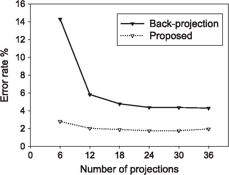

Results of rendered surfaces for setup 2 are shown in Fig. 13. Considerable errors in shape restoration for results of the back-projection method, such as particularly in the leg areas of the mouse, are clearly evident [cf. Fig. 13(c)]. In contrast, these unresolved structures are being better preserved by using the proposed method, as shown in Fig. 13(b).

Fig. 13

Comparison of the rendered surface for the phantom (a), reconstructed surface by the proposed method (b), and the back-projection method (c) from 36 views using setup 2.

4.

Discussion and Conclusion

In the field of in vivo optical imaging, the back-projection method is a frequently used approach for surface reconstruction. This method not only requires a high number of projections (100 to 300 in general) to produce acceptable results,^9,10 but it also possesses inherent shortcomings, mainly regarding its inability to resolve concave areas. Surface reconstruction from multiview projection data using the proposed method has been demonstrated to resolve concave surface areas better. Furthermore, the required number of projections can be significantly reduced when employing MLA-Ds, since MLA-Ds provide additional angular information per detector position. The simulation results indicate that satisfying results can be achieved by 6 to 36 views of projection using the proposed new setup. In contrast to other surface detection approaches used within the research field of in vivo optical imaging, such as using structured light or employing a secondary structural imaging procedure, the approach as proposed in this article does not require any other additional hardware.

Because experimentally acquired data were not available as the final MLA-D construction is still to be completed, results are obtained using the PBRT simulation approach. However, as we run the simulation on highly realistic object data, experimentally acquired by x-ray CT of a nude mouse scan, relying on a simulation study does not degrade its value. By incorporating ray-tracing techniques tailored specifically to the optical layout of the MLA-Ds investigated, the PBRT framework has once more proven to be a state-of-the-art tool for PBRT in computer graphics and, in our context, 3-D in vivo imaging. In addition, we neglected noise in the process of MLA-D image generation mainly due to the fact that the images are acquired under controlled illumination with high signal-to-noise ratio in practice [cf. Fig. 1(b)].

As described in Ref. 22, reference pixel windows were compared with images taken with six closest cameras to calculate the NCC value, which further worked as photo-consistency measure. In contrast to conventional single-lens cameras, MLA-Ds provide multitude EIs covering the same area of interest from (slightly) different views. Hence, a greater number of EIs can be chosen as reference or comparing images and further analyzed to calculate similarity measures. Rather than using the NCC value directly, the proposed measure as described herein combines these inherent characteristics of MLA-Ds by calculating the rate of occasions when the NCC value reaches a maximum at $d=0$. Statistically it uses more information from the neighboring views. However, as $\mathbf{R}(d)$ changes along the virtual optic ray, pairwise comparison of pixel windows from multitude EIs yields very high computational complexity. The calculation of similarity between one pair of pixel windows is independent from the others. Hence, the calculation of photo-consistency could be decomposed into several subtasks and could be further accelerated using parallel computing techniques in the future.

Increasing the number of projectional views does improve the reconstruction results, as seen in Fig. 10; cf. also Ref. 22. The performance of the two setups for 3-D surface reconstruction differs significantly. Because pixel size of setup 2 is about seven times smaller than that of setup 1, setup 2 features a much higher space sampling rate than that of setup 1. Hence, higher-frequency information can be resolved which could potentially make pixel window comparison even more robust. Moreover, the EIs of setup 2 possess higher spatial resolution, such that a bigger pixel window could be used when the similarity measure is calculated. These two advantages are helpful in suppressing false-positive cases in the presence of noise.³³

In conclusion, this article verifies the feasibility of reconstructing 3-D surfaces from multiview data solely by using MLA-D data within the research field of in vivo small animal imaging. We presented a new imaging instrumentation design with respect to the alignment of MLA-Ds and light sources. Given this conceptional imaging system setup, a corresponding algorithm for 3-D surface reconstruction is presented and investigated. The results indicate that the proposed method does have the ability to resolve concave areas and to achieve a high accuracy, even when using a significantly low number of projection views, without the requirement of any additional hardware.